Let your computer play Snake with Reinforcement Learning
Geplaatst op: februari 2, 2023

At Cmotions we love to learn from each other and that is why we regularly collaborate on internal projects, in which we can express our creativity, curiosity and eagerness to learn. In this article we want to share what we did in the ‘Snake’ project, where we learned the computer to play snake using Reinforcement Learning. Never heard of Reinforcement Learning before? Not to worry, we’ll start our explanation of this project at the very beginning. Intrigued by this project and curious what our code looks like, we’ve shared that too!
Introduction
You have learned to walk on your feet when you were only 8-15 months old and before you were two years old you could speak your first small sentences. Your parents’ encouragement was probably an important incentive for you to try to walk after falling. And maybe the ability to reach for other things felt like a victory when you stood on your feet for even a moment and helped you to try it over and over again. Not every time you succeeded, but in the end, you learned how to be stable on your feet and move forward. You learned using Reinforcement Learning! We as humans have amazing learning capabilities and when you dedicate your time and energy in any kind of task you can become extremely good at performing this task. Acrobats, musicians and artists are living examples of human expertise.
As humans we are very skilled at gaining new skills based on what we already learned in the past, we’re quite good at generalizing our knowledge to use in new tasks. But we definitely also have our weaknesses, like we are unable to memorize and process huge amounts of information. That is why we try to program computers to perform these kind of tasks for us. Even though computers have some clear advantages versus humans, it can be difficult to make a computer smart enough to win against a human expert in decision making situations like playing games. In 1996, for the first time, a computer was able to defeat a grandmaster in chess; Kasparov. The computer was able to defeat Kasparov by computing every possible move until there are no more possibilities. This took enormous computing power, but the progress in playing games didn’t end here. Between 2016 and 2019 Computer Algorithms learned to defeat human experts in Go and Chess with a lot less computing power needed. The acceleration in this technology has only grown in the last years with day-to-day implementations such as self-driving cars, robotics and complex strategic games such as Starcraft II and No Limit Holdem Poker. You might wonder how they did this. Well, remember Reinforcement Learning?
Introduction to Reinforcement Learning
When working on trying to defeat the grandmaster of chess, it was quickly recognized that computing all the possible solutions and choosing the best solution is not a very efficient way to play (and win) a game. Reinforcement Learning came to the stage and very soon was able to prove its effectivity when it comes to playing, and winning, games. With Reinforcement Learning the computer learns to make optimal decisions for the future.
The process of Reinforcement Learning looks like this:

In Reinforcement Learning the computer (agent) takes actions within a given set of rules and possibilities (environment). Actions can lead to a positive encouragement (rewards) or negative encouragement (punishments). By taking an action, the agent is moving from one situation (state) to the next. Moreover, the environment holds, in case of chess, the rules of the game like physical size of the board and possible steps per type of piece. In Reinforcement Learning it’s about taking the best possible action or path to gain maximum rewards and minimum punishment in the future through observations in a specific situation.
In the chess game the state of the game would be the situation on the chess board, meaning where each piece is located on the board. This state gives us a possible action space for each piece, meaning all the possible actions at that moment for each piece on the board, of course keeping in mind the rules of the chess game. When the agent (player) moves a piece, the games reaches a new state. Which also means the possible actions for each piece on the board might change as well. Just like when we play chess ourselves, before the computer decides which move to make, it tries to predict what would be the most valuable move, i.e. which move would lead to winning the game as fast as possible.
Let’s see how this would work for chess. The first image shows the start of the game, the first state, for the knight we show its actionspace, but of course each piece of the board has its own. Let’s assume the agent decides to move the knight. Leading to the second image, and second state, of the game. Also meaning the knight, and other pieces, have an updated actionspace.


Of course, at the beginning of a game it can be quite difficult to predict which move would be the most valuable, but as the game progresses, this is becoming more and more clear and easier to predict. Something every chess player will recognize.
In Reinforcement Learning, the agent starts learning by using trial and error. It remembers which moves were made, how long the game lasted and what the outcome was. Like for ourselves, the more we play, the better we know what a good next move would be, giving the current state of the game. But unlike us, a computer can play games at ligthning speed and has a huge memory to remember every little detail.
In more technical terms, in Reinforcement Learning we can use a algorithm which uses the current state and action (next move) as input and expected reward as output. The goal is to find a suitable action model within the environment in which the agent increases the expected cumulative reward of the agent in the future. The expected cumulative future reward is expressed in a value function. Reinforcement Learning models update their value function by interacting with the environment, choosing an action, looking at the new state, looking at the reward, then updating. With multiple iterations the model will keep learning and we expect this value function to increase, meaning the agent will keep improving at playing (winning) the game.
Choosing the right Reinforcement Learning algorithm
In order to teach our agent to take the best actions in all possible states for acquiring the maximum reward over time, we need to choose a Reinforcement Learning Algorithm (RLA) with which our agent can learn what actions work best in the different states.
We call the collection of these preferred actions in the different states the policy of the agent. In the end, the agent should have a policy that will give her the highest lifetime reward. A large variety of algorithms to find the optimal policy exist and we will group them into three categories to make things understandable:
- Model Based
- Policy Based
- Value Based
Model Based
The first category is that of Model-Based RLA’s, where the algorithm uses a model to predict how the environment reacts to actions, thereby giving the agent ‘understanding’ of what her future state will be if she chooses for a particular action. In Model-Free algorithms, the agent will not have an explicit prediction of what her environment will look like after taking an action. So, although every RLA could be seen as a Machine Learning model for the agent to base its actions upon, the distinction between Model-Based and Model-Free is about whether an explicit (predictive) model about the future state is used or not.
Policy Based
Although not explicitly having an expectation of the future environment, some of these Model-Free algorithms can find the ultimate policy, based on searching for an optimal combination of states and wise actions to take in these states. These are called Policy-Based RLA’s. One of the most common algorithms of this sort is the Policy Gradient Method.
Value Based
Some algorithms go one step deeper than these Policy-Based algorithms by optimizing the expected future reward per state. In doing so, these Value-Based algorithms find the best actions to take in these different states, thereby having a collection of state-action combinations which ultimately make up the policy of the agent in her environment. So, Policy-Based and Value-Based algorithms seem very similar, but the main difference is that policies are stored and updated in Policy-Based algorithms, but in Value-Based algorithms the value function is stored and updated, from which the combinations of states and actions can be derived, and the policy thereby constructed. We will be using such an algorithm: Double Deep Q-Network (Double DQN).
Defining the SNAKE game
Now that we know what Reinforcement Learning is and how it teaches an agent to achieve goals by interacting with its environment, it is time to try it ourselves! Remember the game we used to play in the early 2000’s on our good old Nokia mobile phone? We have all been playing the nostalgic game Snake at least once in our life, right? The goal is simple: being a snake you navigate through a square playground looking for food. As you eat more food, the difficulty increases because your snake will grow longer, and you cannot crash into yourself. Snake is a good choice for a first introduction to Reinforcement Learning, because it lets us define the environment, agent, states, actions and rewards relatively simple.
Our game environment can be defined as a grid of points, with a piece of food at a random coordinate in that grid. In our version of Snake there are no walls, which means that the only way the snake can die is by a collision into its own body. Our agent – the snake – is encoded by a list of coordinates that are covered by the snake, and the state is the current representation of the environment. The picture below shows an example of what the environment could look like. Where the F is food, H is the head of the snake and T is its tail.

For this article, we have experimented with different representations of the state, incorporating various sources of information such as the direction of the snake and the distance to the food. Additionally, we have experimented with adding spatial features extracted by convolutional filters. Convolutional filters extract spatial information of an image by multiplying regions of pixels in an input with weights that are learned by a neural network. This results in a feature mapping that encodes spatial information of the playground, like we will explain more in detail later on.
As the snake navigates through the environment, it can either move up, down, left or right. However, according to the rules of the game, the snake cannot move in the opposite direction of the current direction. Therefore, given the state, we can only take three out of four actions. This subset of actions is what we call the action space. Our goal is, given a certain state, to choose the action that maximizes the future lifetime reward, which can consist of multiple features. In the first place, our snake is rewarded when it eats food, and the score increases. Conversely, the snake is negatively rewarded when it collides into its own body. Additionally, we have included a small penalty to the reward when the snake moves further away from the food, and we added a small positive reward when the snake moves closer to the food. This encourages the snake to pursue eating food instead of only avoiding a collision.
It is very informative to play around with these rewards and punishments, since the result of your decisions on what to reward and what to punish might surprise you from time to time (actually, a lot of the times). For example, before introducing the small rewards and punishments for getting closer to or moving away from the food, the snake would sometimes run in circles in order to survive, thereby not scoring any points. On the contrary, a penalty for walking around for too long without eating, resulted in the snake wanting to commit suicide immediately to avoid “suffering” from walking around without eating. Taking into account how simple the game of snake is, imagine how hard it is to define good rewards and punishments in real life, to avoid “toxic” behaviour.
Now that we know what the actions, rewards and states in our situation are, it’s time to have a look at how we are going to incorporate this in a model that can be trained.
Optimizing Reinforcement Learning
By using a neural network with Python library Tensorflow we estimate the total future rewards of our possible actions given our state. So, given a set of input features, which is the current state, we are going to predict the future rewards given our possible actions. In other words, we are training our neural network by updating our Q function based on the reward for a given action. Such a neural network is called a Deep Q-Network (DQN). This Q-function is the prediction of total future reward for the agent, when choosing action a in state s. The formula representing the way the function is updated is called the “Bellman-equation” and given by:

So, besides the Q function, the equation has parameter alpha as the learning rate of the algorithm that influences how fast the Q function is updated and therefore the rate at which the perception of the agent changes while learning her best actions. Reward function R shows the immediate reward of taking action a in state s. Discount rate gamma discounts future rewards that come after the immediate reward. This is necessary to reflect real life, in which a reward in the far future is most of the times deemed (slightly) less important than immediate reward. These hyperparameters alpha and gamma are set by the programmer before the algorithm is deployed.
By learning which actions give us the most future reward in which states, the agent can learn to effectively play snake.
We are going to train two different models with different input features/states in order to compare the performance and complexity of both versions.
Model V1 – a simple model
The first step we must take in building a DQN model is to define the features/states that we will use to predict the Q-values. This is one of the most important steps in setting up a Reinforcement Learning model as it yields all the information the model will use, such that giving too little information will result in a poor model performance. Nonetheless, we do not want to overcomplicate our first model and therefore choose fairly simple input features that contain signals about the location of the food and if there is a snake cell (i.e. her own body) beside the head of the snake.
For the first model we tried to keep the features as easy as possible to understand for our neural network (and ourselves 😉). The features used by this first model are as follows:
- X-coordinate of the food minus the x-coordinate of the snake’s head.
- Y-coordinate of the food minus the y-coordinate of the snake’s head.
- Dummy variable: if there is snake cell below head
- Dummy variable: if there is snake cell above head
- Dummy variable: if there is snake cell left of head
- Dummy variable: if there is snake cell right of head
Based on these features we give the snake information about the location of the food, and immediate danger of a certain choice based on the snake’s body. However, the snake does not have full information about her body and therefore cannot strategically choose actions to avoid being locked by her body later in the game.
For this first version of the model, we insert fairly simple input features that consist of ‘which direction the food is’ and ‘if the snake’s body is near its head’, we do not want to overcomplicate our model. Therefore, we choose to build a neural network consisting of two layers with 16 neurons and end with a dense layer that forecasts the reward for each action. This neural network will then be used as our Q function.
Once the model is set, we want to train the model until it converges to an optimum, which means that we do not see the average reward improve anymore (enough) after a certain number of training iterations. We help the model converge quicker by giving example actions for 20% of the time. This way, the model has enough data about how to gain rewards such that these actions will gain higher Q-values.
For our first version of the model, we find that after around 500.000 training iterations, we don’t see the rewards improve anymore. This takes around 30 to 60 minutes of training, depending on the processor speed.

Model V2 – a more strategic model
As we chose our first model to be fairly simple, it could not look further ahead on the snake’s body to understand the full current state of the game and therefore the snake could be trapped easily inside its body such that it dies. To improve the model, we want to use a convolutional neural network to understand the full picture of the game such that it can make strategic choices so that it will not trap itself.
However, by using convolutional filters to understand the game’s image there is a tradeoff between simplifying the input by aggregating the pixels of the game, such that it will lose precision on the whereabouts of the snake’s body, and size of the network such that the network can understand the many pixels given by the image, where a too large size will make the model so complex that it will take very long to train.
To deal with this problem we create a combined network of the input features from the last model, that gives very precise information about dangers and directions, and combine them with the snake’s snapshot image such that it will give the snake more strategic insights about the state of the game.
In order to let the neural network understand the image, we transform the game into an array of shape: (game width, game height, 3). This array will then have an array with the length of three for each point in the snake’s map, that will be used to indicate if there is a snake body, snake head or food by using dummy variables. For example, if the pixel is filled with a snake’s body, the array will then be given by [1,0,0] and if there is food placed on the pixel the array will be given by [0, 0, 1]. Then, an example of what the full input array for the convolutional layers could be is given by:

Now the input of the DQN model for this version will be a tuple with the state features of our first model’s version and the game state array for the convolutional part of the model. Because of this combination of two parts, it is a Double DQN.
As previously mentioned, the input of the model will be a combined input of model V1 on features and the image as converted to an array. Our model will first split our tuple containing both features by the features array and the convolution array. Once we have our separated array containing the snake’s game snapshot, we will let this go through two separate convolutional layers containing 8 filters, a kernel with size=(4, 4) and strides=2, where the padding is ‘same’ which makes sure that we also account for the border pixels in our model. After the input has gone through both convolutional layers, we will have extracted signals about the game like “there are a lot of body parts in the bottom right corner”, which can help the snake to stay away from there. Flattening this array of signals makes us able to use these signals in a normal dense layer. Next, after flattening the array, we use two dense layers of 256 and 64 neurons to further extract signals about the state of the game.
For the normal features we use one dense layer of 16 neurons to extract signals about immediate threats and the position of the food. The moment comes when we concatenate both the normal signals and our convolutional signals together such that we can use them simultaneously in a dense layer which will finally be used to predict the Q-values for each action.
Next, we train our multi-input model until the model converges to an optimum where the average reward is not improving anymore. As we have a much larger network containing convolutional filters, it will take the algorithm a lot longer to train. Again, we help the model by giving example actions for 20% of the time. Once the model has had a good amount of training loops (around 1 million iterations) this part can be removed to get more exploration observations and have more data to find a good strategy in the training data.
For this second version of the model, we find that it converges after approximately 5 million training iterations which take around 4-7 hours of training, depending on the processor speed.
Results
Finally, we come to the most important part of the project where we assess the performance of our models. To validate the performance, we want our models to play 100 games till the snake dies. Then we are going to compare the average score and the maximum score out of these 100 games to compare the models. Exploration is avoided, which means that the algorithm is never randomly choosing actions. These are the results:
| Score | V1 Model | V2 Model |
|---|---|---|
| Avg Score | 22.28 | 27.16 |
| Max Score | 47 | 72 |
For the model V1 the average score out of 100 games is 22.28 with a maximum of 47 which is not bad for the fact that this model is not able to lookout for threats ahead. However, incorporating the snapshot of the whole game into the model V2 gave us a significant improvement with an average of 27.16 and a maximum of 72. This shows us that the V2 model, the more strategic one, is indeed capable of determining strategies that look ahead to prevent the snake from getting trapped. However, the training time of this model was also significantly longer with 4-7 hours in respect to 30 to 60 minutes. Therefore, we really see a clear trade-off between performance and required training time to reach the optimum. In practice, this is always a hard decision as there is always a better solution, however the question arises: “Is it worth the time?”. From our first model’s output we saw that the performance was not bad either, so was it worth all the trouble to enhance it? For this article it definitely was!
Can you use Reinforcement Learning in your daily life?
Apart from interesting applications of Reinforcement Learning in games, these algorithms can also be used in business to improve how data can create value. Essentially, if decisions must be made about which actions to take given the current situation an organization is in, a Reinforcement Learning agent can be trained to make decisions or at least give advice on what the next best action should be.
One of these scenarios could be when a marketing team should decide whether to include a customer or prospect in a certain campaign and which offer or communication she should receive. For example, the agent here is the digital assistant of the marketeer, state the characteristics of the (potential) customer plus the timestamp and the actions are choosing between the different offers (or no offer at all) and communications. The environment, which is the real world, will give feedback such as clicks on weblinks, conversion or churn. The designer of the Reinforcement Learning Algorithm should then define the rewards corresponding to these events to steer the agent in the right direction for finding its optimal policy.
Another example could be that of personalizing the homepage on a website based on how a visitor is navigating through the website. The agent is not the visitor, but the digital content manager behind the website, who is choosing which banners to show on which places of the homepage (actions), given online navigation history (states) of the visitor and other information if the visitor is logged in with a profile or from cookies. If the visitor clicks on the shown banner, a positive reward is given by the environment, as this click shows the banner is relevant to the visitor and the homepage is being optimized for this type of visitor. The algorithm will find which actions (show a banner) link best to the possible states (collection of navigation history) to compose the policy.
Curious to see our code for both the Reinforcement Learning models, check out our other article!


Building a Beatles lyrics generator
Geplaatst op: december 7, 2022

In 1964, the Beatles released their iconic song “I Want to Hold Your Hand”. Since then, the Fab Four have become one of the most influential bands in music history. Now, fifty years later, you can generate your own Beatles lyrics using AI. In recent years, artificial intelligence (AI) has made significant advances in the field of natural language processing (NLP), which has resulted in the development of AI systems that can generate human-like text. One application of this technology is the generation of text and music lyrics using AI.AI-generated text is not just a gimmick; it has a variety of applications in the real world. For example, AI can be used to generate product descriptions, blog posts, and even music lyrics. In this article, we’ll take a look at how AI can be used to generate text, with a focus on music lyrics.
Human or machine generated text
This is actually the first paragraph we wrote ourselves. The text above was all written by an algorithm called GPT-3 by Open AI by instructing it to write an article about generating text for Beatles songs. With the recent release of Chat-GPT the introduction of this article can even be improved. Over the last 20 years, text analytics has really taken off (as the AI already said). Where 20 years ago analyzing your customer satisfaction research using word counts was state of the art, and google translate was completely literal, and therefore often nonsensical, nowadays it actually gives you valid output. Text analytics on customer satisfaction surveys or reviews can now help you derive the drivers and the sentiment of your customers. That way you can really improve your satisfaction or NPS by identifying actionable insights. You can train your chatbot by having it read all your F.A.Q.’s and help pages. This will improve the relevance of the answers the chatbot is giving to its users.
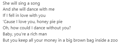
In terms of text generation, have you noticed how good Whatsapp can predict what you are typing? Or how accurate the suggestions of Outlook are on how to respond to your email? With its foundation in deep learning algorithms and its increasing computing power text generation has really taken a flight in the last 5 years. This has been driven in part by the development of neural networks, which are a type of AI that is designed to mimic the way the human brain learns. With this technique we trained an algorithm to speak “Beatle”. Based on an input prompt, it creates Beatles lyrics for you, complete with a title and cover. Curious what this looks like? Take a look at the following example below or try it yourself:

Showcase our demo on Hugging Face spaces
Using Hugging Face, a datascience platform and community that provides many integrated tools to build, train or deploy models based on open-source code, we fine-tuned a pre-trained model to behave “Beatles-like” with some additional training on the original Beatles lyrics. Besides that, a pre-trained summarization model is used to create a matching title. And finally, a deep learning, text-to-image model is used to create the song cover. We demo the result of our efforts in a Hugging Face Space. These spaces are integrated with Gradio, a tool that wraps a python function so it can be launched almost anywhere: a jupyter notebook, a colab notebook, on your own website or hosted on a Hugging Face Space.
Evaluate our model
All of us are by no means ‘Professors in Beatleness’. To judge to what extent our model to generate Beatly lyrics is any good, we’ve set up an evaluation plan. Evaluating NLG models is not that obvious: There is no ‘ground truth’ to compare the generated lyric with. In our blog on evaluating NLG models, we explain different methods to evaluate these types of models. And we apply some of them to our own lyrics. Our approach is twofold: use popular metrics to evaluate NLG models and ask Beatles fans their honest opinion on our ‘Beatly’ (or not so ‘Beatly’) lyrics.
This evaluation results in some interesting insights: Popular evaluation metrics indicate that our model is performing quite well. Both BLEURT and BERT-score reported an f-score higher than 0.7 which indicates that the generation quality of our songs was decent. However, we also asked a critical crowd of Beatles fans what they think of the lyrics we generated. Based on their input it was less evident that the generated songs are that Beatly because of good evaluation metrics. This shows that human judgement is still important as well, as they pointed out to us that some lines in the generated songs literally come from original Beatles songs. In general, the reviewers were not that convinced that AI is ready to replace their beloved Beatles. Of course, we do have to take into account that real Beatles fans are less prone to agree their heroes are actually replaceable, so some bias might be presented there as well. To conclude, AI is able to do impressive things, also in the domain of generating texts. When you have a use case to create a natural language generation model of your own, we hope our series inspires you how to approach this. It shows how you can benefit from Huggingface’s great repo and spaces to host your model so you can enable others to test and use your model. And we’ve shown how different evaluation approaches can and need to be used to get a good view of the quality of your NLG solution.
- In this blog you can read details on how the demo our work in a Hugging Face space
- Read this blog to find out how we evaluated the quality of a fine-tuned text generation model for Beatles-like lyrics


How to showcase your demo on a Hugging Face 🤗 space
Geplaatst op: december 7, 2022

Natural Language Processing is a subfield of Artificial Intelligence and has already existed for some time. Recent years, there have been many developments and nowadays not only human language can be analyzed, but it can also be generated by AI models. There are several so-called language models able to generate human-like texts. Probably the most well-known example is GPT-3, which is created by OpenAI. This model shows the current possibilities for language generation.
The impressive possibilities of GPT-3 made us start a project to learn more about language generation. Our goal is to use an existing language model and finetune it for another task. The Hugging Face 🤗infrastructure seems to be the best way to go for this project. At Cmotions we are a big fan of the Hugging Face infrastructure and services. This data science platform and community provides many integrated tools to build, train or deploy models based on open-source code. In general, it is a place where engineers, scientists and researchers gather to share ideas, code, and best practices to learn, get support or to contribute to open-source projects. In short, Hugging Face is the “home of machine learning”.
The main focus of Hugging face is on Transformers, a platform that provides the community with APIs to access and use state-of-the-art pre-trained models available from the Hugging Face hub. You can make use of existing state-of-the art models resulting in lower computing costs and a smaller carbon footprint. If you are looking for either high performance natural language understanding and generation or even computer vision and audio tasks this is the place to go.
Models that you have trained or datasets that you have created can be easily shared with the community on the Hugging Face Hub. Models are hosted as a Git repository with all the benefits of versioning and reproducibility. When you share a model or dataset to the hub it means that anyone can use it, eliminating their need to train a model on their own. Isn’t that great! As a bonus sharing a model on the Hub automatically deploys a hosted Inference API for your model, a sort of instant demo.
Our Beatles project
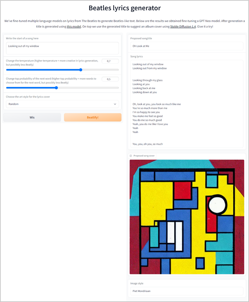
Now back to our project, what did we do? We wanted to see if we could train an already existing language model in a way that it could produce Beatles-like text, maybe even Beatles-like songs! First, we searched for language models that could be used. From the Hugging Face Hub we chose to use GPT-Medium, GPT-Neo-125m and the Bloom-560m model, which are already trained language models by Hugging Face users. To teach these pre-trained models how to behave we required additional training on Beatles lyrics. Therefore, we created a dataset with all Beatles lyrics and fine-tuned our models. The newly trained models were put on the Hugging Face Hub, so that we could use these for our text generation, and the community as well. With these models, we were able to generate lyrics based on an input prompt. We evaluated several models to see which settings gave the best result. In the figure below, an example of a generated text is shown.
But what are song lyrics without a song title? So we extended our scope and based on a summarization model ‘story-to-title‘ we created a title for the generated lyrics as well. This model created by Caleb Zearing is based on a T5 model and trained on a large collection of movie descriptions and titles. This model proved valuable for our Beatles song titles: when given generated lyrics it will generate a corresponding title.
Only one thing was missing then: a song cover. Wouldn’t it be great if we could generate an album cover image based on the title? With the introduction of so-called Stable Diffusion models a text-prompt can be used to generate a detailed image. Stable Diffusion is a deep learning, text-to-image model released in 2022. It is primarily used to generate detailed images conditioned on text descriptions, though it can also be applied to other tasks such as inpainting, outpainting, and generating image-to-image translations guided by a text prompt.
Put it all together on a Hugging Face space
When you are ready to show the world what you have made, Hugging Face Spaces makes it easy to present your work. These Spaces are great to showcase your work to a non-technical audience. In our case we’ve used the Gradio library to build our demo. Gradio wraps a python function into a user interface and the result can be launched within a jupyter notebook, a colab notebook, on your own website or hosted on Hugging Face Spaces.
We want to combine the lyrics, title and cover generation function into a good-looking interface, and Gradio has all we need to showcase what we have done. In the example code snippet below we simple call the Gradio Interface creation.
gr.Interface(fn=generate_beatles
             , inputs=[input_box, temperature, top_p, given_input_style]
             , outputs=[gen_title, gen_lyrics, gen_image, gen_image_style]
             , title=title
             , css=css
             , description=description
             , article=article
             , allow_flagging='never'
             ).launch()
The function that is used is the function we made to generate the lyrics, title and cover. The inputs consist of the input prompt, some model parameters and a list to choose from for the style of the album cover. Lastly, the type of output is defined. That is all there is to it. Our Beatles lyrics demo can be found here, as well as the code to reproduce it.
How to evaluate a text generation model: strengths and limitations of popular evaluation metrics
Geplaatst op: december 7, 2022

The purpose of this article is to provide a comprehensive description of evaluation methods that can be applied to a text generation task. Three different evaluation techniques are introduced, then used to analyze lyrics written in the Beatles’ style.
With the evolution of technology, language models are continually evolving in sync with technological developments. With these developments, Natural Language Generation (NLG) allows us to create models that can write in human languages. More than you may be aware, a lot of the applications we use daily—like chatbots, language translation, etc.—are based on a text generation model. Building these language models to be “as human as possible” is difficult since numerous factors, including linguistic structure, grammar, and vocabulary, must be considered.
An important challenge in developing models that can generate human level text is to assess how closely the text generated by your model compares to humans. In this blog we show some popular evaluation metrics you can use and what their strengths and limitations are.
The unsupervised nature of these tasks makes the evaluation procedure challenging. However, it is vital to determine whether a trained model performs well. The most frequently used approaches for these tasks are: Human judgment, Untrained Automatic Metrics, and Machine-Learned Metrics. The following overview is based on a survey on evaluation of Text Generation.
Human judgment
As this model is trying to write in human languages and produce a text that is valuable to people, the best way to validate the output is human based. In this scenario you can have multiple people review the model and give insight into how well the model is performing. This can be done with an annotation task; this method provides the readers with a guideline that describes how they can proceed with the evaluation. Even though this type of evaluation is considered important, there are multiple limitations. Human evaluations can be time consuming and expensive, often the amount of data reviewed is large so therefore, it is difficult for an individual to manually inspect the content. Also, the judgments by different annotators are prone to be ambiguous, resulting in unreliable assessment of the quality of the text generating model. Inter-annotator agreement is therefore an important measure of the model’s performance. This metric indicates whether the task is well-defined and the differences in the generated text are consistently noticeable to evaluators. However, this evaluation method is biased since the assessed quality of the model also depends on the personal beliefs of each annotator. Therefore, this can lead to the evaluation results being subjective.
Based on these limitations, different ways of evaluating language models such as NLG have been developed. To minimize costs involved with the manual judgment and to have less ambiguity in judging generated texts, automated metrics have gained popularity to evaluate NLG models.
Untrained Automatic Metrics
With the implementation of untrained automatic metrics, the effectiveness of language models can be calculated. These methods can be used to calculate a score that contrasts an autonomously generated text with a reference text that was written by a human. Utilizing these techniques is simple and efficient. There are many different automatic measures, including metrics for n-gram overlap, distance-based metrics, diversity metrics, and overlap metrics for content. For this blog we are going to focus on n-gram overlap metrics.
N-gram overlap metrics are commonly used for evaluating NLG systems. When you are trying to evaluate a generated text your first instinct may be to figure out the similarity degree to the human reference to assess the quality of the generated text. And that is exactly what this type of metric does. The overlap between these two texts is calculated with the number of subsequent words from a sequence (n-gram). Some well-known metrics that are based on this approach are: bilingual evaluation understudy (BLEU), Recall-Oriented Understudy for Gisting Evaluation (ROUGE), Metric for Evaluation of Translation with Explicit Ordering (METEOR).
Despite their popularity, these metrics do have some big drawbacks. Most importantly, these metrics are sensitive to lexical variation. This means that when other words with the same meaning are used, the model will be punished since the text will not be the same. As they only look at the overlap using unigrams and bigrams, the semantic and syntactic structure is not considered. For example,[1] if we have the sentence ‘people like foreign cars’ – this type of evaluation will not give a high score to a generated sentence such as ‘consumers prefer imported cars’ and will give a high score to ‘people like visiting foreign countries’. When semantically correct statements are penalized because they vary from the reference’s surface form, performance is underestimated.
The true semantics of an entire sentence cannot be evaluated using n-gram based metrics. Therefore, machine learning metrics emerged to find a way to measure text with higher qualities.
Machine-learning based metrics
These metrics are often based on machine-learned models, which are used to measure the similarity between two machine-generated texts or between machine-generated and human-generated texts. These models can be viewed as digital judges that simulate human interpretation. Well-known machine learning evaluation metrices developed are BERT-score and BLEURT. BERT-score can be considered as a hybrid approach as it combines trained elements (embeddings) with handwritten logic (token alignment rules) (Sellam, 2020). This method leverages the pre-trained contextual embeddings from Bidirectional Encoder Representations from Transformers (BERT) and matches words in candidate and reference sentences by cosine similarity. Since that is quite a mouth full, let’s break that down a bit: Contextual embeddings generate different vector representations for the same word in different sentences depending on the surrounding words, which form the context of the
target word. The BERT model was one of the most important game changing NLP models, using the attention mechanism to train these contextual embeddings. BERT-score has been shown to correlate well with human judgments on sentence-level and system-level evaluations. However, with this approach there are some elements that need to be considered. The vector representation allows for a less rigid measure of similarity instead of exact-string or heuristic matching. Depending on the goal or ‘rules’ of the project this can be a limitation or an advantage.
Finally, another machine learning metric is BLEURT, a metric developed using BERT for developing a representation model of the text and relies on BLEU. The selection of the appropriate evaluation method depends on the goal of the project. Based on the project and the component generated some of these methods can be considered strict or lenient on the results. Therefore, it might be the case that the evaluation scores are high or low because the evaluation metric chosen is not the right one.
Let’s apply some of these metrics to a concrete example: As you can read in our previous blog posts we’ve trained an NLG model to write lyrics in the style of the Beatles. Obviously, we’re anxious to learn whether our model is doing a good job: are we actually Beatly? Based on the results generated by the two machine learning evaluation metrics, it seemed that our model was performing quite well. Both BLEURT and BERT-score reported an f-score higher than 0.7 which indicates that the generation quality of our songs was decent.
However, we already mentioned that quantitative metrics like BLEURT and BERT-score have some deficits. Therefore, we also asked a critical crowd of Beatles fans what they think of the lyrics we generated. To collect human observations, a questionnaire was generated. In this questionnaire 15 songs were used, 12 generated by our model and 3 originals. This survey was then posted on a social media platform that contains thousands of Beatles fans and were asked to let us know what they think of the made-up songs. Based on these results it was evident that the generated songs were not as good as the machine-based scores presented them. Some of the fans even characterized these songs as “awful” or “written poorly”. The readers also pointed out a good observation, apparently our models often repeat existing Beatles lyrics, which defeats the purpose of text generation. We do have to consider that Beatles fans are less prone to agree their heroes can be replaced by AI, so some bias might be presented there as well… In conclusion: With the evolvement of technology, the Natural Language Generator has made a great contribution in our daily lives. The unsupervised nature of the model makes the evaluation process challenging. To minimize costs involved with the manual judgment and to have less ambiguity in judging generated texts, automated metrics have gained popularity to evaluate NLG models. However, machine learning evaluations metrics can be seen to fall short in replicating human decisions in some, even in many circumstances. These metrics are not able to fully cover all the qualitive components of generated text. Therefore, a human in the loop is still needed most of the time. It is worth noting that human judgment observation can result to a biased interpretation based on the subjective interpretation of the reader.
[1] This example was sourced by 1904.09675.pdf (arxiv.org)
First time right with NLP: zero shot classification
Geplaatst op: november 13, 2022

Is your Power BI report slow? Let’s fix that
Geplaatst op: oktober 31, 2022

In this blog I explain how you can improve the performance of your Power BI report. For a long time I was struggling with a bad performing report I used for a training. Now I finally found the solution I’m happy to share my insights with you.
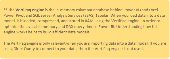
So if your Power BI report is running slow or you want to avoid it to run slow, you probably should optimize your data model. This is usually where the most performance gains can be made. Reducing the memory of your model has a direct impact on the performance of your reports and dashboards. To find out which optimizations potentially have the most impact, you need information about the used memory in your data model. VertiPaq*1 analyzer is the tool to accomplish this. This tool is available on sqlbi. Personally I prefer the version which is integrated in DAX Studio.
In this blog I work with an example database called ‘Mrbean’. It holds data on customers and their orders for a fictive coffee retailer in the Netherlands.
Perform an analysis
Open your report in Power BI desktop. Then launch DAX Studio (from the external tools tab) to perform an analysis of the used memory in your data model.
Within DAX Studio select View Metrics (Advanced tab) to perform the analysis (you have to be connected to a model (Home tab > Connect). The results will be discussed in the next section.

It is also possible to generate a VPAX file in DAX Studio (use Export Metrics). This file has a very limited size and can be shared easily. Making it possible to do a (quick) analysis of a model of which you can’t access the PBIX file.
Interpret the results
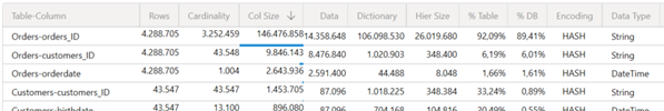
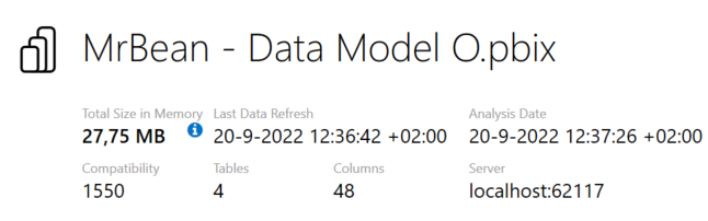
Before you start investigating the results, first look at the summary tab. Here you’ll find the total in memory size of your model in MB. In the example the model is 160 MB, which is pretty large.

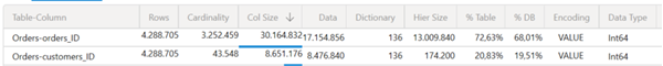
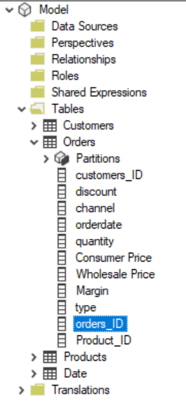
The tables tab provides an overview of the tables in the data model. The total size of each table is displayed. As well as how much a table is taking up as percentage of the total size of all tables. In this example the Orders table accounts for 95% of the total size. By expanding the view of the Orders table it becomes clear the orders_ID column is the primary cause. This is also shown on the columns tab, which gives an overview of the most expensive columns in the database.

Performance optimalisation steps
Based on the results of the analysis I took the following 5 steps to optimize the model.
- Disable auto date/time
If the table overview shows tables starting with LocalDateTable auto date/time is enabled. Meaning Power BI generates hidden calculated tables for each date column in your model. These tables increase the model size. Therefore it is better to create your own date table and disable this file setting. In this example this saves only 4 MB (2,5%), but the impact can be much bigger.

- Choose the right datatype for a column
Vertipaq is datatype independent. Therefore it doesn’t matter if a column has a text, bigint or float data type. Vertipaq needs to create a dictionary for each of those columns. The size of this dictionary determines the performance, both in terms of speed and memory space allocated.
Since the orders_id column has the largest share in the size of the model this is the place to start optimizing. It is a string column with many distinct values. This means low compression. Vertipaq uses the hash algorithm *2 to store the data. Resulting in a large dictionary size (106 MB). This is being referred to as a high cardinality.
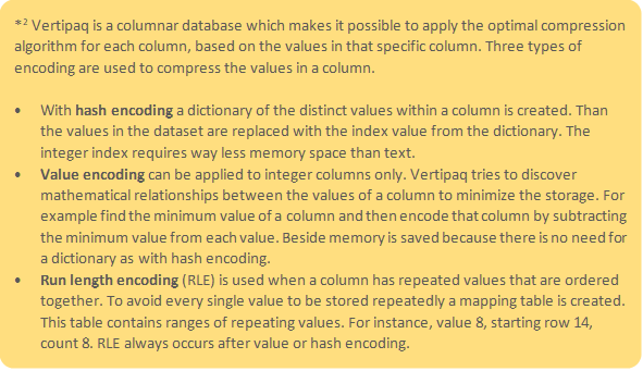
With an integer datatype value encoding may be enabled. This is why I converted the orders_ID column to an integer. I replaced the store (S) and webshop (W) indicator in the orders_ID with a number. Unfortunately what I expected did not happen. There was no change in dictionary size. Hash encoding is still applied to compress the column, because the orders_ID values fluctuate significantly within the range (81.000 to 9.999.990).
To overcome this problem I created an index column based on the orders_ID. This change was made in the data source. Now the number range is smaller (1 to 3.252.459) and the numbers linearly increase. Making VertiPaq assume that it is a primary key and choose value encoding. This has a major impact on the size of the data model. The dictionary of 106 MB disappears and the hierarchy size decreased tremendously (13 MB). Resulting in a way smaller model size of 45 MB.

Enabeling the right encoding is also applicable for other columns. The customers_ID column in the Orders table also consumes a considerable amount of memory. This is an integer column stored as text. After changing the datatype value encoding is enabled. However, because the customers_ID has a lot of digits the size to store the data remains high. Replacing the customers_ID column with an index column in the Orders and Customers table in the data source solves this problem. Saving another 3 MB in model size.
- Selecting the appropriate decimal features
If your decimal numbers have a precision of four or fewer decimals it is recommended to use the fixed decimal number data type. This data type is internally stored as an integer and therefore can be stored more efficiently. Applying this to several columns (i.e. wholesale price, consumer price, margin and discount) saved 1 MB in the data model.
- Remove unnecessary columns
A logical step in optimizing your data model is to remove the columns you don’t need. Especially the ones with a high column size. Don’t let the thought that you potentially might need a column later stop you. If you remove a column in the Power Query editor you can always undo this later. In this example birthday is not needed, because there is also an age column available. For the geographical analysis the customers region is needed, so latitude, longitude and city are not needed. Finally customer type can be removed from the orders table, because it is a customer property already available in the customers table. Bringing the total model size to 40 MB.
- Set available in MDX to false
Another way to optimize your model is by looking at the size of the automatically generated hierarchy of a column (used by MDX). These hierarchies are used to improve the user experience in Excel and other client applications that use the MDX query language against tabular models and Power BI datasets. The size can be set to zero in Tabular Editor by changing the option available in MDX to false. After applying this option to the columns with the largest hierarchy size (orders_ID and customers_ID), the model size decreased to 28 MB.
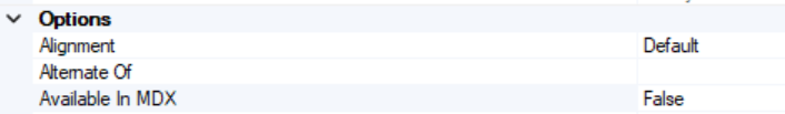
Within Tabular Editor select a column an go to the options menu on the right, here you can set Available In MDX to False
The result
The 5 performed optimization steps resulted in a saving of 82,5%. The performance problems I often faced during my trainings with this dataset now disappeared.
Learnings when working on this article
- After performing optimization steps in Power Query editor you have to close and re-open the PBI file in order to see the real size of the data model. Otherwise the string columns will default have an allocated size of 1MB. Making you think that your optimizations steps didn’t make the expected impact.
- Sometimes all properties of a column seem to be fitted for value encoding, but Vertipaq still uses the hash algorithm. Changing the encoding hint setting in Tabular Editor to value may help to solve this problem. In order to be able to change this setting you’ve to select the allow unsupported Power BI features (experimental) option within preferences (in the file menu).
- Sometimes encoding settings changed after I made changes to columns used in a relationship. Value encoding switched back to hash encoding bringing the dictionary size back to the model. When I created the relationships in the data model after performing all optimization steps this behavior didn’t occur.
Useful links
https://www.sqlbi.com/
https://www.alphabold.com/brain-muscles-of-powerbi/
https://towardsdatascience.com/how-to-reduce-your-power-bi-model-size-by-90-76d7c4377f2d

Interactive geovisualization in Python using Bokeh
Geplaatst op: oktober 28, 2022


An in-depth Introduction to Topic Modeling using LDA and BERTopic
Geplaatst op: oktober 21, 2022


If you are interested in the evolution of technology when it comes to text mining tools and Natural Language Processing tasks, then you are in the right place! This article presents one of the most well-known NLP tasks: topic modeling. We are providing a thorough overview of topic modeling techniques as well as an in-depth discussion of two different topic models. In this post we are presenting a traditional approach, Latent Dirichlet Allocation (LDA) and a deep learning method, BERTopic. If you also would like to see these models in practice, we also generated topic modeling notebooks implementing the different approaches mentioned (BERTopic and LDA).
Let us set the scene, imagine entering a bookstore to buy a cookbook and being unable to locate the part of the store where the book is located, presuming the bookstore has just placed all types of books together. In this case, the importance of dividing the bookstore into distinct sections based on the type of book becomes apparent[1]. Topic Modeling is a process of detecting themes in a text corpus, like splitting a bookstore depending on the content of the books. The main idea behind this task is to produce a concise summary, highlighting the most common topics from a corpus of thousands of documents. This model takes a set of documents as input and generates a set of topics that accurately and coherently describe the content of the documents. It is one of the most used approaches for processing unstructured textual data, this type of data contains information not organized in a pre-determined way. Over the past two decades, topic modeling has succeeded in various applications in the field of Natural Language Processing (NLP) and Machine Learning. Throughout the years this task has been used in various domains such as airlines, tourism and more. You might be wondering, what is the value of this task to a business? Well, let me tell you!
The rapid development of technology has contributed to developing new technological tools to improve many domains such as Customer Experience (CX). As customer experience can be crucial in maintaining a successful business, many organizations have adapted to newly developed technological tools. Among the tools used for analyzing and improving customer experience, a significant amount is within the field of Natural Language Processing (NLP), such as topic modeling. Different types of data contain meaningful information for a company’s objectives, such as reviews, customer and agent conversations, tweets, emails, etc. To fully understand clients’ needs, companies must use a wide range of technological tools to analyze which characteristics impact customer experience and satisfaction. In business settings, topic modeling insights can improve a company’s strategy and assist in developing marketing platforms.
History of Topic Modeling
Topic modeling emerged in the 1980s from the ‘generative probabilistic modeling’ field. Generative probabilistic models are used to solve tasks such as likelihood estimates, data modeling, and class distinction using probabilities. The main idea behind this task is to produce a concise summary highlighting the most common topics from a corpus of thousands of documents. This model takes a set of documents as input and generates a set of topics that accurately and coherently describe the content of the documents. Topic models are continually evolving in sync with technological developments. As a result, new topic modeling techniques have been developed since the 1980s.
It is worth noting that not all topic modeling techniques can be used and are suitable for all types of data (Churchill and Singh[2], 2021). For example, the algorithm used to retrieve hidden topics on social media data might not perform well for scientific articles due to the different patterns of words. Each data and domain characteristic, such as document length, and sparsity, must be considered before implementing a topic modeling algorithm (Churchill and Singh, 2021). In this scenario sparsity can be identified as two different kinds: model and data sparsity. Model sparsity means that there is a concise explanation for the effect we are aiming to model. While data sparsity is bad as there is missing information and the model is not observing enough data in a corpus to model language accurately. Data sparsity is an issue within the field of NLP as it concerns a great number of vocabularies. Due to this variation of different types of data, new topic modeling approaches are developed.
In this article we are going to present two different methods that can be used for implementing a topic modeling task. One method is a traditional model while the second one is a new deep learning approach. We are going to compare and discuss the limitations that need to be taken into consideration when implementing the models.
Latent Dirichlet Allocation (LDA)
Latent Dirichlet Allocation (LDA) is a three-level hierarchical generative model. This model is a powerful textual analysis technique based on computational linguistics research that uses statistical correlations between words in many documents to find and quantify the underlying subjects (Jelodar et al.,2019). [3]This model is considered state of the art in topic modeling.
‘Latent’ represents the process of the model to discover the hidden topics within the documents. The word ‘Dirichlet’ indicates that the distribution of subjects in a document and the distribution of words within topics are both assumed to be Dirichlet distributions. Finally, ‘Allocation’ represents the distribution of topics in the document (Ganegedara, 2019). For a deeper understanding of the components within the LDA topic model a blog written by Thushan Ganegedara [4]offers a great explanation.
The model implies that textual documents are made up of topics, which are made up of words from a lexicon. The hidden topics are ‘a recurring pattern of co-occurring words’ (Blei, 2012)[5]. Every corpus that contains a collection of documents can be converted to a document word/document term matrix (DTM). LDA converts the documents into DTM, a statistical representation describing the frequency of terms that occur within a collection of documents. The DTM gets separated into two sub-matrices: the document-topic-matrix: which contains the possible topics, and the topic-term-matrix: which includes the words that the potential topics contain (Seth, 2021)[6].
Parameters
This topic modeling approach can be implemented in various ways, but the model’s performance comes down to specifying one or more parameters. The most crucial parameters, in this case are the following: Number of topics: the optimal number of topics extracted from the corpus, Alpha: controls prior distribution over the topic weights across each document and Eta: controls prior distribution over word weights across each topic. Depending on the data as well as the goal of the task a grid search needs to be executed to find the optimal parameters. A grid search is a tool used for exhaustively searching the hyperparameter space given in an algorithm by trying different values and then picking the value with the best score. If you think that this topic modeling approach is interesting and would like to further observe the implementation of the technique, then we got you! We generated a notebook that executes a topic modeling task using LDA.
BERTopic
Devlin et al. (2018)[7] presented Bidirectional Encoder Representations from Transformers (BERT) as a fine-tuning approach in late 2018. If the first thing that comes to mind when reading the word Transformers is the movie, then you might want to look at a blog written by Jay Alammar [8]before continuing with this article. A variation of Bidirectional Encoder Representations from Transformers (BERT) has been developed to tackle topic modeling tasks. BERTopic was developed in 2020 by Grootendorst (2020) [9]and is a combination of techniques that uses transformers and class TF-IDF (term frequency-inverse document frequency) to produce dense clusters that are easy to understand while maintaining significant words in the topic description. This deep learning approach supports sentence-transformers model for over 50 languages for document embedding extraction (Egger and Yu, 2022)[10]. This topic modeling technique follows three steps: document embeddings, document clustering and document TF-IDF.
Parameters
As with any other language model, BERTopic also has some parameters that need to be taken into consideration. The values assigned to these parameters are crucial as they have a major influence on the performance of the model. Some parameters are the Number of topics: the optimal number of topics extracted from the corpus, Language: the primary language used in the training data and Embedding model: depending on the domain of the data, an embedding model needs to be used. There are several numbers of different parameters but in this article the most important ones were presented. This deep learning method gives the user the opportunity to replace all components withing the parameters. For example, the user can select the embedding mode, dimension reduction method with the preferred one. Depending on the task executed and the desired goal, changing the defaults might influence and improve the predictive performance and topic quality of the model. If you would like to see how a BERTopic model is implemented, or if you would like to experiment on different parameters you can find our notebook here ’link for notebook’.
LDA Vs BERTopic
In this article we presented two different ways that an individual can use to execute a topic modeling task. Before you decide which one you would like to use there are some limitations as well as advantages that need to be taken into consideration before implementation. Let us look at the positive side of these models first!
LDA is considered as a state-of-the art topic detection technique, it is a time efficient method. For context, the size of the data used for this project was 11314 documents, when implementing the topic model, the training procedure took less than five minutes. Moreover, this generative assumption confers one of the main advantages, LDA can generalize the model it uses to separate documents into topics to documents outside the corpora. Even though the time efficiency and generative assumption of the model are crucial factors there are also some disadvantages that are crucial for the performance of the model. The first drawback of this generative model is that it fails to cope with large vocabularies. Based on previous research, executors had to limit the vocabulary used to fit and implement a good topic model. This can lead to consequences for the performance of the model. To restrict the vocabulary usually, the most and least frequent words are eliminated; this trimming may remove essential terms from the scope (Dieng et al.,2020)[11].
Another significant limitation is that the core premise of LDA is that documents are considered a probabilistic mixture of latent topics, with each topic having a probability distribution over words, and each document is represented using a bag-of-words model (BOW). Based on this approach, topic models are adequate for learning hidden themes but do not account for a document’s deeper semantic understanding. The semantic representation of a word can be an essential element in this procedure. For example, for the sentence ‘The man became the king of England’, the representation of a bag of words will not be able to identify that the word ‘man’ and ‘king’ are related. Finally, when the training data sequence is altered, LDA suffers from ‘order effects’ which means that different topics are generated. This is the case due to the different shuffling order of the training data during the clustering process. Any study with such order effects will have systematic inaccuracy. This inaccuracy can lead to misleading results, such as erroneous subject descriptions.
Due to these limitations, many new generative and deep learning models have been generated using this traditional approach as a base to improve the topic quality and predictive performance. One of those improved models is BERTopic. This approach, as mentioned before, can take into consideration the semantic understanding of the text with the use of an embedding model, and generate meaningful topics of which the content is semantically correlated. In the case of a topic modeling task, it is vital to produce topics that are correlated and understandable to a human. This deep learning approach does not have any limitations concerning the size of the data used for the task. This prevents the concern of removing essential terms from the scope. Moreover, with this approach it is possible to use multilingual data as there is an available parameter called ’language’ when training the model. Finally, as the model uses embedding models it is possible for the user to choose from a wide variety of embedding models or even create their own custom model. This model has improved some aspects of traditional methods, but it does not mean that there are no limitations that need to be taken into consideration for this algorithm.
When it comes to topic representation, this model does not consider the cluster‘s centroid. A cluster centroid is ‘a vector that contains one number for each variable, where each number is the mean of a variable for the observations in that cluster. The centroid can be thought of as the multi-dimensional average of the cluster’ (Zhong, 2005)[12]. BERTopic takes a different approach, it concentrates on the cluster, attempting to simulate the cluster’s topic representation. This provides for a broader range of subject representations while ignoring the concept of centroids. Depending on the data type, ignoring the cluster’s centroids can be a disadvantage. Moreover, even though BERTopic’s transformer-based language models allow for contextual representation of documents, the topic representation does not directly account for this because it is derived from bags-of-words. The words in a subject representation illustrate the significance of terms in a topic while also implying that those words are likely to be related. As a result, terms in a topic may be identical to one another, making them redundant for the topic’s interpretation (Grootendorst, 2022). Finally, an essential disadvantage of BERTopic is the time needed for fine-tuning, for this project an hour was needed for this model to train.
Concluding Remarks
This article presented two different approaches to topic modeling. LDA is a generative model which categorizes the words within a document based on two assumptions: documents are a mixture of topics and topics are a mixture of words. In other words, ‘the documents are known as the probability density (or distribution) of topics, and the topics are the probability density (or distribution) of words. While BERTopic is a deep learning method which takes into consideration the frequency of each word t is extracted for each class i and divided by the total number of words w. This is a form of regularization of frequent words in the class, then the total number of documents m is divided by the total frequency of word t across all classes n. As a result, rather than modeling the value of individual documents, this class-based TF-IDF approach models the significance of words in clusters. This enables us to create topic-word distributions for each document cluster.
You might be wondering, but when should I use LDA and when BERTopic? Well, this decision depends on many factors. For example, the size of the data and the resources used for the task can be crucial for the decision of which model is better. If an individual is working with a great amount of data and their resources are not powerful enough, then it can be the case that topic model takes a tremendous amount of training time. Then in this case the way to go is LDA is the way to go. Or if an individual thinks that the semantic representation of their data is important and would like to take it into consideration then BERTopic is the solution. At the end of the day, it really depends on the goal and target of the project. When it comes to tuning the topic models for the best result, LDA takes a great amount of time in terms of tuning and preparing the input. For example, inspecting the data, pre-processing, and filtering. While in the case of BERTopic many different variants can be tested, such as which pretrained model to implement for embeddings, what dimension reduction and clustering techniques to use.
The main aim of this article was to introduce topic modeling and highlight the importance of retrieving hidden topics within a great amount of text data. Moreover, give a summary of the history of topic modeling as well as the models that have been created with technological development. Finally, this article aims to show the value of an NLP task such as topic modeling, therefore two notebooks were also generated to give a better overview of the practical matters of implementation (BERTopic and LDA). This automatic topic retrieval can provide a company with information about the most frequent matters that the customers talk about and improve a company’s strategy and assist in developing marketing platforms.
If you enjoyed reading this article and you would like to know more about NLP and the variety of tasks that it includes, check out our series Natural Language Processing.
[1] This example was inspired by Topic Modelling With LDA -A Hands-on Introduction – Analytics Vidhya
[2] The Evolution of Topic Modeling (acm.org)
[3] [1711.04305] Latent Dirichlet Allocation (LDA) and Topic modeling: models, applications, a survey (arxiv.org)
[4] Intuitive Guide to Latent Dirichlet Allocation | by Thushan Ganegedara | Towards Data Science
[5] Probabilistic topic models | Communications of the ACM
[6] Topic Modeling and Latent Dirichlet Allocation (LDA) using Gensim (analyticsvidhya.com)
[7] [1810.04805] BERT: Pre-training of Deep Bidirectional Transformers for Language Understanding (arxiv.org)
[8] The Illustrated Transformer – Jay Alammar – Visualizing machine learning one concept at a time. (jalammar.github.io)
[9] BERTopic (maartengr.github.io)
[10] (PDF) A Topic Modeling Comparison Between LDA, NMF, Top2Vec, and BERTopic to Demystify Twitter Posts (researchgate.net)
[11] [1907.04907] Topic Modeling in Embedding Spaces (arxiv.org)
[12] [PDF] Efficient online spherical k-means clustering | Semantic Scholar
Topic Modeling with Latent Dirichlet Allocation (LDA)
Geplaatst op: oktober 21, 2022

If you would like to read more about Topic Modeling, please have a look at our article ‘An in-depth Introduction to Topic Modeling using LDA and BERTopic‘ and make sure to check out the notebook generated based on a deep learning approach, BERTopic.
If you are in general interested in NLP tasks then you are in the right place! Take a look at our series Natural Language Processing.