Complete Azure DevOps CI/CD guide for your Azure Synapse based Data Platform – part II
Geplaatst op: juni 23, 2023

I wrote an article recently describing how to implement Continuous Integration and Continuous Deployment (CI/CD) for your Azure Synapse based data platform. At the end of part one we setup the infrastructure required for CI/CD, and we did our first parameterized deployment from our development environment to the production environment.
In part two we are going to focus on specific use cases to make our CI/CD process completer and more robust.
Situation
We have just setup our first Azure DevOps CI/CD pipeline for our Azure Synapse based Data Platform (Preferably with the help of part 1). It does the job well, but we run into some limitations that are that not immediately obvious to solve. Specifically, two uses cases; what to do with our triggers that should behave differently between our development and production environment, and what to do with our serverless SQL databases which is currently not easy to deploy to production.
Dynamically adjust triggers between your development and production environment
It is likely that you want different triggers running your Synapse pipelines in the development and production environment. Azure Synapse has the functionality to start and stop triggers, meaning when a trigger is stopped it will not run the pipeline it is attached to. This gives us the opportunity to start and stop certain triggers in development and production. This is important because of multiple reasons. For example, we do not want to run our development pipelines at the same time as our production pipelines because of workload constraints.
Luckily, we can automate the process of starting and stopping triggers. We can toggle the triggers on or off in our Azure DevOps pipeline, we do this by adding an extra task to our YAML file. The following code will stop all the triggers in our development environment.
- task: toggle-triggers-dev@2
  displayName: 'Toggle all dev triggers off'
  inputs:
    azureSubscription: '${{ parameters.subscriptionDev }}'
    ResourceGroupName: '${{ parameters.resourceGroupNameDev }}'
    WorkspaceName: '${{ parameters.synapseWorkspaceNameDev}}'
    ToggleOn: false
    Triggers: '*'
Code snippet 1: Stopping all triggers in dev
It is worth paying attention to the specific value for “Triggers”. In the example above we give it the wildcard value “’*’” which means that all the triggers in development environment will be stopped. We could also give it some hard coded names of triggers that we want to stop, as seen in code snippet 2.
- task: toggle-triggers-dev@2
  displayName: 'Toggle specific triggers off'
  inputs:
    azureSubscription: '${{ parameters.subscriptionDev }}'
    ResourceGroupName: '${{ parameters.resourceGroupNameDev }}'
    WorkspaceName: '${{ parameters.synapseWorkspaceNameDev}}'
    ToggleOn: false
    Triggers: 'trigger1,trigger2,trigger3'
Code snippet 2: Stop specific triggers
In this example, only the triggers called trigger1, trigger2, and trigger3 will be stopped. This solves some of our problems, because we can now toggle the production triggers in the production environment by adding them to the list. The same applies to the development environment. However, this would mean that we always need to adjust our Azure DevOps pipeline when we create new triggers, which is not an ideal situation. That is why we need to go one step further and automate this process.
We start with naming conventions for our triggers. We name every trigger in our development environment that needs to be started “_dev” and every trigger in our production environment that’s needs to be started “_prd”. Now we have something that we can use to recognize the environment the trigger is meant for. Unfortunately, at the time of writing this article, it is not possible to use some kind of string recognition in our “Triggers” parameter, we need to give it exact names of the triggers. That is why we need a workaround.
In order the get the correct list of triggers, we are going to use a PowerShell script which we will run in the Azure DevOps pipeline in replacement of the task we described above.
$triggers = az synapse trigger list `
              --workspace-name ${{ parameters.synapseWorkspaceNameDev}} `
              --query "[].name"
foreach ($trigger in $triggers) {
    if ($trigger.Contains("_dev")) {
      $trigger = $trigger.Trim() -replace '[\W]', ''
      az synapse trigger start `
        --workspace-name ${{ parameters.synapseWorkspaceNameDev }} `
        --name $trigger
    }
}
Code snippet 3: Starting triggers dynamically in development
First, we create a variable named “triggers” which will contain a list of all the triggers in our development environment. We achieve this by using the Azure CLI. Make sure to add “—query “[].name”” to only get the names of the triggers. Next, we are going to loop over this list with a for each loop and check for every trigger in the list if it contains “_dev”. If this is the case, we make sure that there is no whitespace in the name of the trigger and then we run an Azure CLI command to start this trigger. This way all the triggers in with “_dev” in their name will be started.
We run this PowerShell script using an Azure CLI task in our YAML file.
#Start triggers in dev synapse environment
- task: AzureCLI@2
  displayName: 'Toggle _dev triggers on'
  continueOnError: false
  inputs:
    azureSubscription: '${{ parameters.subscriptionDev }}'
    scriptType: pscore
    scriptLocation: inlineScript
    inlineScript: |
      $triggers = az synapse trigger list `
        -–workspace-name ${{ parameters.synapseWorkspaceNameDev}} `
        --query "[].name"
      foreach ($trigger in $triggers) {
          if ($trigger.Contains("_dev")) {
            $trigger = $trigger.Trim() -replace '[\W]', ''
      az synapse trigger start `
       --workspace-name ${{ parameters.synapseWorkspaceNameDev }} `
       --name $trigger
          }
      }
Code snippet 4: Azure DevOps pipeline task to run PowerShell script
The same can be done for our production environment. By using the naming conventions in combination with the PowerShell script we can now automatically and dynamically start and stop triggers in our Azure Synapse environments. We do not need to manually add triggers to our Azure DevOps pipeline, but we only need to stick to our naming conventions, which will hopefully result in less bugs.
How to deal with your serverless SQL pool?
At the moment of writing this blog Microsoft does not have an out of the box solution for automatically deploying our serverless databases and associated external tables from our development to our production environment. Therefore, we use a pragmatic and quite easy solution to solve this limitation.
In this example we are going to focus on creating external tables on our data which we need in our production environment. The external tables are not automatically deployed using the Azure DevOps pipeline, therefore we need a workaround. We can do this by manually creating a migration pipeline in our development Synapse workspace.
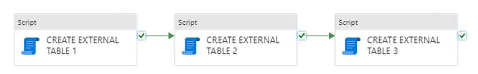
Figure 1: Example of migration pipeline
As an example, I have created three Script activities in the pipeline which all contain a SQL script to create external tables on the existing data. We already ran these scripts in our development environment, but we want to also run them in our production environment.
Since we do not want to do this manually, we need to find a way to automate this. We will do this by adding the following task at the end of our Azure DevOps deployment pipeline.
#Trigger migration pipeline
- task: AzureCLI@2
  condition:  eq('${{ parameters.triggerMigrationPipeline }}', 'true')
  displayName: 'Trigger migration pipeline'
  inputs:
    azureSubscription: '${{ parameters.subscriptionPrd }}'
    scriptType: pscore
    scriptLocation: inlineScript
    inlineScript: |
      az synapse pipeline create-run `
        --workspace-name ${{ parameters.synapseWorkspaceNamePrd }} `
        --name ${{ parameters.migrationPipelineName }}
Code snippet 5: Azure DevOps pipeline task to trigger migration pipeline
After the synapse workspace is fully deployed to our production environment, this task will trigger the migration pipeline we just created. We run the migration pipeline by executing an Azure CLI command “az synapse pipeline create-run” where we specify the Synapse workspace name and the name of the migration pipeline. By running this pipeline in our Synapse production environment, we ensure that the external tables are created in the production serverless SQL pool.
As you can see, we added a condition to the task which states this task will only run if our parameter “triggerMigrationPipeline” is set to “true”. By adding this to our CI/CD pipeline, we can trigger the migration pipeline in our production environment only if we want it to.
In the example above we focused on creating external tables in the serverless SQL database, but the migration pipeline can be used for multiple purposes. For instance, if we have pipelines which need a special initialization to run properly, we can put those initialization activities in our migration pipeline. For example, creating a stored procedure that is used in our pipeline. In summary, we can put all the activities we need to make sure that the triggered pipelines are going to run without any errors in the migration pipeline to make sure everything is initialized.
If you are looking for a more complete version of implementing CI/CD for your serverless SQL pool, you can check out this blog by Kevin Chant, in which he uses a .NET library called DbUp.
Summary
The use cases discussed above will make your CI/CD process more dynamic and robust. By dynamically adjusting triggers between your environments and adding a migration pipeline to migrate your serverless databases, you will have less manual work when deploying to your production environment. Of course, there are more automation possibilities and uses cases to further enhance your CI/CD process for your Azure Synapse based data platform, and with the development of the Microsoft stack, we will get new possibilities to make our lives easier.
If you would like more in-depth code or contribute yourself, check out: https://github.com/atc-net/atc-snippets/tree/main/azure-cli/synapse/Publish.


Princess Peach rescued from the claws of Bowser at our Super Mario Hackathon
Geplaatst op: mei 3, 2023

At 21 april 2023, we held an epic hackathon where 10 teams from KPN, Rabobank, DPG, Athora, ANWB, UWV, Lifetri, and Eneco joined forces to rescue our beloved Princess Peach from the claws of Bowser. It was a fierce battle, but in the end, only one team emerged victorious. And who was that, you may ask? It was none other than the heroic team from UWV! Congratulations, heroes!
But let’s not forget all the other teams who participated. You all showed great courage and skill, and we thank you from the bottom of our hearts. It was truly an adventure we’ll never forget.
Now, without further ado, we present to you the amazing aftermovie of this epic hackathon, created by none other than Jan Persoon. Check it out below, and relive the excitement!
But wait, there’s more! We’re already hard at work preparing for our next hackathon of 2024, so keep an eye on our social media channels for updates. In the meantime, enjoy the aftermovie and let it inspire you for your next adventure.
Until next time, may the stars guide your path!


Let’s get balanced! A simple guide on how to deal with class imbalance in your binary data
Geplaatst op: april 17, 2023

At Cmotions we’ve always had a lot of discussion amongst colleagues whether or not to balance our datasets when building a predictive model. Everyone has their own personal preference and way of working, but which approach is “the best”? We simply didn’t know until we stumbled upon this paper written by Jacques Wainer and Rodrigo A. Franceschinell in October 2018. Unlike a lot of other research papers, this paper focuses on the practitioners (us) and not so much on researchers, since in general, a practitioner has a couple of days or weeks to build a model on a dataset, while a researcher may spend several years working with the same dataset. Because not everybody likes to dive into scientific papers, I’ve tried to summarize their conclusions in this blog as best I can.
Research setting
Let’s start with the setting of the research:
- Binary classification problems
- 82 datasets
- The datasets were altered (if possible) to have an imbalance between 0.1% (severe) and 5% (moderate)
- Focus on strong general classifiers:
- Focus on easy to implement balancing strategies:
- Baseline: no balancing
- Class weight: assign more weight to the small class, the general setting used here is that the large class has a weight of 1 and the small class a weight of the inverse of the imbalance rate. Thus, if this rate is 1% the weight of the small class would be 100
- SMOTE (synthetic minority over-sampling): use KNN to find neighbours of the small class to randomly create a new data point for this class
- Underbagging: bagging of the base classifier, where each instance is trained on a balanced sample of the dataset, where the small class is preserved and the large class is randomly undersampled. This strategy has a parameter n, the number of sampled datasets created, in this research they used n as a hyperparameter to find the best value for each dataset
- Focus on most used metrics (in research):
- Area under the ROC curve (AUC): the estimated probability that a random positive example will have a higher score than a randomly selected negative example
- Accuracy (acc): the proportion of correct predictions
- Balanced accuracy (bac): the corrected accuracy based on the caculation of the arithmetic mean of the recall (the proportion of true predictions for the positive examples) and specificity (the proportion of true predictions for the negative examples)
- F-measure (F1): the corrected accuracy based on the harmonic mean of recall and specificity
- G-mean (gmean): the corrected accuracy based on the geometric means of recall and specificity
- Matthew’s correlation coefficient (mcc): the Pearson correlation between the prediction and the correct class
The researchers mainly made these choices based on what we as practitioners have in our most-used-toolbox. For myself, I can support this for most of the decisions. Although I must say, I very rarely use SVM.
The key take aways when looking at these settings:
- The lowest class imbalance is 5%, which is considered moderate in this paper, thus more balanced datasets are not taken into account here
- This only holds for binary problems and not multiclass
- The researchers chose to use strong general classifiers on purpose, since we would use them in practice too, just keep in mind this affects the extent to which the balancing strategy has an effect on result, since some of these classifiers are able to deal with imbalancing to some extent
Research questions
In this paper Wainer and Franceschinell answer multiple questions, we will focus on the five questions that are most relevant to us. Which leads down to determining the best balancing strategy in general, for a given metric and if the data is severely or moderately imbalanced. They’ve also looked at which classifier works best with which balancing strategy or without using any balancing strategy. All questions we as Data Scientists have to think about every time we are building a predictive model.
If in the tables below multiple answers are given for the same metric, keep in mind that the order given is random, since the difference will be insignificant so we can’t order them based on that.
What is in general the best strategy for imbalanced data (for each metric)?
| Metric | best performing Balancing strategy |
| AUC | Baseline | Class weight |
| acc | Baseline | Class weight |
| bac | Underbagging |
| f1 | SMOTE |
| gmean | Underbagging |
| mcc | Baseline | Class weight | SMOTE |
What is the best balancing strategy for moderately (5%) imbalanced data?
| Metric | best performing Balancing strategy |
| AUC | Baseline | Class weight | SMOTE |
| acc | Baseline | Class weight |
| bac | Underbagging |
| f1 | SMOTE |
| gmean | Underbagging |
| mcc | SMOTE |
What is the best balancing strategy for severely (0.1%) imbalanced data?
| Metric | best performing Balancing strategy |
| AUC | Baseline | Class weight |
| acc | Baseline | Class weight |
| bac | Underbagging |
| f1 | Baseline | Class weight | SMOTE | Underbagging |
| gmean | Underbagging |
| mcc | Baseline | Class weight | SMOTE | Underbagging |
What is the best combination of base classifier and balancing strategy?
| Metric | best performing Balancing strategy |
| AUC | RF + Baseline | RF + SMOTE | RF + Class weight | XGB + Baseline | XGB + Class weight | XGB + SMOTE |
| acc | XGB + Baseline | XGB + Class weight | RF + Class weight | | RF + Baseline |
| bac | XGB + underbagging |
| f1 | XGB + SMOTE |
| gmean | RF + Underbagging | XGB + Underbagging |
| mcc | XGB + SMOTE |
What is the best base classifier when not using as balancing strategy?
| Metric | best performing Balancing strategy |
| AUC | RF | XGB |
| acc | RF | XGB |
| bac | XGB |
| f1 | XGB |
| gmean | XGB |
| mcc | XGB |
Conclusion
The first conclusion will probably be no surprise for most of us. The XGB classifier is a very strong and stable classifier, which performs better than the other classifiers in most use cases.
The next conclusion surprised us a lot more. We never expected that balancing data isn’t even necessary in most cases, let alone that it is even less necessary if your data is severely imbalanced.
The last conclusion is the fact that the best balancing strategy strongly depends on the metric chosen to evaluate the model performance. Which would mean that we should base our balancing strategy on the metric we think is the best to use in a given use case. Unfortunately, this is never an easy decision to make, as it depends on a lot of factors.
These are the guidelines given in the papers conclusion about this:
- If the user is using AUC as the metric of quality then baseline or class weight strategies are likely the best alternatives (regardless if the imbalance is moderate (5%) or severe (0.1%). If the practitioner has control over which base classifier to use, then one should opt for a gradient boosting or a random forest.
- If one is using accuracy as metric then baseline or class weight are the best strategies and the best classifier is gradient boosting.
- If one is using f-measure as metric then SMOTE is a good strategy for any imbalance rate and the best classifier is gradient boosting.
- If one is using G-mean as metric then Underbagging is the best strategy for any imbalance rate and the best classifiers are random forest and gradient boosting.
- If one is using Matthew’s correlation coefficient as metric then almost all strategies perform equally well in general, but SMOTE seems to perform better for less imbalanced data and the best classifier is gradient boosting.
- If one is using the balanced accuracy as metric then Underbagging is the best strategy for any imbalance rate and best classifier are random forest and gradient boosting.
How do we use this in our day-to-day work
You might wonder, did this settle all our discussions for once and for all? To be honest, not really, since we just love to debate and question every decision we make. That is how we make sure we keep growing and learning. But it did help us a lot in our daily work.
The biggest insight for most of us was that balancing the data is often not even necessary, and the most counterintuitive is that this is even more the case for severely imbalanced datasets.
The biggest change for me actually had nothing to do with choosing the right balancing strategy, but with more deliberately picking a metric (or a couple of metrics) when evaluating a model. When it comes to picking a balancing strategy my own preferred way of working is still to simply try a couple of balancing strategies and evaluating all of the resulting models coming from this. Maybe some of you are horrified by this, but it works for me.
What is your prefered way of working when it comes to choosing a metric and/or choosing a balancing strategy? I’m always looking for people who can convince me to change my habits 😉
Opening the Black Box of Machine Learning Models SHAP vs LIME for model explanation
Geplaatst op: februari 28, 2023


Complete Azure DevOps CI/CD guide for your Azure Synapse based Data Platform – part I
Geplaatst op: februari 28, 2023

This guide includes code snippets which you can use yourself. Credits to my colleagues at Delegate who have contributed a lot to this domain. If you would like to check out more extensive CI/CD code or contribute yourself check out: https://github.com/atc-net/atc-snippets/tree/main/azure-cli/synapse/Publish.
You have setup your synapse workspace and are busy developing your data platform, there are already some reports that make use of that data platform. You receive some complaints from the analysts that your development work is causing problems for the reports depending on the output of the data platform. You conclude that it is time to separate the development environment from the production environment. You want a professional approach and automate deployment to production in a structured way. Continuous Integration and Continuous Development (CI/CD) is the perfect way to automate your deployment process, but you don’t know where to start.
No worries, this guide will help you from beginning to end with implementing CI/CD for your Azure Synapse based data platform. In this first part we will take a deep dive into CI/CD with Azure DevOps and in the second part we will highlight some of the best practices.
Azure DevOps CI/CD process for your Synapse data platform
We start with a high-level overview of the CI/CD architecture in figure 1. This is the architecture that we are going to setup, but before we can set up this architecture we need to make some assumptions.

Figure 1: CI/CD architecture for Azure Synapse with Azure DevOps
- You have an organisation, project and repository ready to go in Azure DevOps in the same tenant as your Synapse workspace.
- You have one development Azure Synapse workspace and one empty production Azure Synapse workspace. In this guide we are going to assume that these are in different subscriptions, but this does not have to be the case (although it is recommended).
- You have two service principals (app registrations) in your Tenant, one for each of the subscriptions. Find out more about Application and service principal objects in the Microsoft documentation.
- These service principals need to have Contributor permissions on the resource group in order to create azure resources in their dedicated subscription.
- An Azure Active Directory (Azure AD) administrator must install the Azure DevOps Synapse Workspace Deployment Agent extension in your Azure DevOps organization. You can find out how you can install extensions in the following link.
In order to continue with this guide, the assumptions need to be met or at least take them in consideration while reading the guide.
Connect your Azure Synapse workspace to an Azure DevOps repository
Before we can start implementing CI/CD we need to make sure that the Azure Synapse workspace is connected to your Azure DevOps repository, which will result in the DevOps branches shown in figure 1. The advantage of setting up the connection between Azure Synapse and Azure DevOps is that we can use Git for source control and versioning. We can set this up by going through the following steps.
- Navigate to your Azure Synapse Workspace and select “manage” from the left-side menu.
- Select “Git configuration” and “configure”.
- Select the option “Azure DevOps Git” from the dropdown menu in “Repository type”
- Choose the correct tenant which contains the Azure DevOps organisation and project.
- Choose your DevOps organisation, project and repository which you already setup.
- Create a “Collaboration branch” which will be your development branch.
- The “Publish branch” will contain the JSON file which defines your Synapse workspace and will be updated when you press publish (we will come back to this later on).
- Make sure the box beneath “Import existing resources” is checked. This will make sure that everything that you have built up to this point is pushed to the repository.
- Select “Apply”
You now have successfully connected your Synapse workspace to your Azure DevOps workspace and we can continue with setting up your Azure DevOps environment.
Create service connections in Azure DevOps to your Azure subscriptions
In order to automatically deploy the Synapse workspace from development to production we need to authenticate and authorize. We will be doing this using Azure service connections which make use of service principals in Azure (in figure 1 these are the lines between the Synapse workspaces and the DevOps resources). We already have a service principal with the sufficient rights for each subscription. The following steps will describe how we can access and use these service principals in Azure DevOps.
- Go to your project settings at the bottom in the left-side menu of Azure DevOps.
- Navigate to “service connections” beneath the header “Pipelines” and select “New service connection” in the top right corner.
- Choose the option “Azure Resource Manager”.
- Next choose the option “Service principal (manual)”.
- Select the option “Subscription” for the scope level and fill in the correct subscription id. You can find the subscription Id in the Azure Portal under subscriptions.
- Fill in all the required fields. Remember we are going to create a service connection for both the development and production requirement, so make sure you select the corresponding service principal.
- Select Verify to test if the connection works.
- If the connection works, give a name to the service connection, make sure to include the environment in the name (so development or production).
- To finish up select “Verify and save”.
We need to repeat these steps twice, once for development and once for production. When you went through the steps for both development and production, you will be able to authenticate and authorize automatically when deploying to your Synapse workspace.
Create your first Azure DevOps Pipeline
Now we can continue creating our Azure DevOps Pipeline. We will first create a starter pipeline which will serve as the starting point for our deployment pipeline. We will create this starter pipeline using the Azure DevOps UI, which will result in a YAML file. We will expand this YAML file during the rest of this guide.
- Log into your Azure DevOps environment and go to the repository where you connected your Synapse workspace.
- Go to the main branch.
- Select “Pipelines” in the left-side menu and select “New pipeline” in the top-right corner.
- Select “Azure Repos Git YAML” and select your repository.
- Configure your pipeline as a “Starter pipeline”.
- You will now see the YAML file, select “Save and run”.
Your starter pipeline will now run. You can click on “Job”, now you will see the steps that the YAML file is performing. Let’s take a closer look at the YAML file.
trigger:
- main

pool:
  vmImage: ubuntu-latest

steps:
- script: echo Hello, world!
  displayName: 'Run a one-line script'

- script: |
    echo Add other tasks to build, test, and deploy your project.
    echo See https://aka.ms/yaml
  displayName: 'Run a multi-line script'
Firstly, the trigger of the pipeline is defined, the pipeline will trigger when the main branch is updated. Secondly virtual machine (VM) on which the pipeline runs is specified, the pipeline runs on a Linux VM with the latest ubuntu distribution. Next, the steps of the pipeline are defined. The starter pipeline contains two steps which both run an inline shell (Bash) script. Step one prints “Hello, world!” and the second step prints two strings in the shell. You can see that the second step contains “displayName” parameter which is used to give a step a descriptive name. When you run the pipeline you will see a step with the name “Run a multi-line script”.
Deploy a Synapse workspace with your Azure DevOps pipeline
Now that we have a starting point for our deployment pipeline we can start configuring the YAML file to our needs. We will start with deploying our development Synapse workspace to our production Synapse workspace. This will only be a “simple” copy paste action on which we can build.
We will start with adding some parameters to the file.
parameters:
- name: subscriptionPrd
  type: string
  default: service-connection-prd

- name: subscriptionDev
  type: string
  default: service-connection-dev

- name: resourceGroupNamePrd
  type: string
  default: resource-group-prd

- name: resourceGroupNameDev
  type: string
  default: resource-group-dev

- name: synapseWorkspaceNamePrd
  type: string
  default: service-connection-prd

- name: synapseWorkspaceNameDev
  type: string
  default: service-connection-dev
We start with the parameters for the service connections to both the development and production subscriptions. These will make sure we can authenticate and authorize. Next, we have the names for our development and production resource groups and Synapse workspaces.
We talked about the workspace_publish branch in the previous section, we will now further elaborate on this branch. Our development Synapse workspace is defined in the workspace_publish branch which is automatically created when you connect your Synapse workspace to Azure DevOps. This branch contains two JSON files; “TemplateForWorkspace.json” and “TemplateParametersForWorkspace.json”. The first file contains the complete definition of our Synapse workspace and the second file contains global parameters in the Synapse workspace. We will be adjusting the parameter file later on, for now we will be doing a simple deployment where we just copy the development environment to the production environment.
resources:
  repositories:
  - repository: PublishBranch
    type: git
    name: 'name of your repository'
    ref: workspace_publish

steps:

- checkout: PublishBranch
  path: PublishBranch
We need these files in order to deploy to our production environment. Therefore, we need to make sure that we can access the files during deployment. In the code above we add the “workspace_publish” branch as resource to our pipeline. In next we checkout the “the workspace_publish” branch so that we can make changes to the files if needed, we will come back to this later on.
Now we can finally implement the most important step, deploying the Synapse workspace in our production environment.
#Deploy synapse production environment
- task: Synapse workspace deployment@2
  continueOnError: false
  displayName: 'Deploy Synapse Workspace'
  inputs:
    operation: 'deploy'
    TemplateFile: '$(Agent.BuildDirectory)/PublishBranch/main/TemplateForWorkspace.json'
    ParametersFile: '$(Agent.BuildDirectory)/PublishBranch/TemplateWorkspaceParameters.json'
    azureSubscription: '${{ parameters.subscriptionPrd }}'
    ResourceGroupName: '${{ parameters.resourceGroupNamePrd }}'
    TargetWorkspaceName: '${{ parameters.synapseWorkspaceNamePrd}}'
    DeleteArtifactsNotInTemplate: true
This task will execute our Synapse workspace deployment. First, we specify that this task must not be executed if we get any errors in the previous steps, to make sure we don’t deploy faulty code. In the input parameter we specify the definition of our Synapse workspace. In the “Templatefile” parameter we will refer to the “TemplateForWorkspace.json” file in our checked out “publishBranch”. We will do the same for “ParametersFile”. Because we are deploying to our production Synapse workspace we will authenticate and authorize with our production service connection in the “azureSubscription” parameter. To make sure our development and production environment stay aligned we include the “DeleteArtifactsNotInTemplate” parameter and set it to true. This setting will delete everything in the production Synapse workspace that is not defined in the “TemplateForWorkspace.json” file that we deploy.
When we now run the Azure DevOps Pipeline we will deploy our development Synapse workspace to our production Synapse workspace in an automated way. We will continue with parameterizing our deployment to production.
Parameterizing the deployment to production
Because our development Synapse workspace is in a different environment than our production Synapse workspace we need to make some adjustments to our parameters. For example, we have a connection string to a storage account. The connection string will be different in the production environment, because we want to connect to a different storage account. The “TemplateParametersForWorkspace.json” file contains key value pairs where we need to replace the value. We will use the adjusted “TemplateParametersForWorkspace.json” file with the replaced values in our deployment step.
Let’s walk through the process. First we are going to create a new folder in our main branch root and name it “deploy”. In this folder we are going to create a JSON file named “synapse-parameters.json”. This file contains the key value pairs of the parameters we would like to replace in our “TemplateParametersForWorkspace.json” file, for example:
{
    "workspaceName": "synapse_workspace-prd",
}
Next we create a PowerShell file in the “deploy” folder and name it “initialize-synapse-parameters.ps1”. This file contains the following code:
function Initialize-SynapseParameters {
    param (
        [Parameter(Mandatory = $true)]
        [ValidateNotNullOrEmpty()]
        [string]
        $SynapseParameterJsonPath,

        [Parameter(Mandatory = $true)]
        [ValidateNotNullOrEmpty()]
        [string]
        $OutputPath,

        [Parameter(Mandatory = $true)]
        [ValidateNotNullOrEmpty()]
        [string]
        $ParameterJsonPath
    )

    # Get the Synapse generated Parameters file
    $synapseParameters = Get-Content -Raw $SynapseParameterJsonPath | ConvertFrom-Json -AsHashTable

    Write-Host "Parameterize using jsonfile: $ParameterJsonPath" -ForegroundColor Yellow
    $parameterUpdates = Get-Content -Raw $ParameterJsonPath | ConvertFrom-Json -AsHashTable

    foreach ($parameter in $parameterUpdates.GetEnumerator()) {
        $synapseParameters.parameters.$($parameter.Name).value = $parameter.Value
    }

    # New re-parameterized file ready for prod
    Write-Host "Saved parameterized workspace file at: $OutputPath"
    $synapseParameters | ConvertTo-Json | Out-File "$($OutputPath)"
}

Initialize-SynapseParameters `
  -OutputPath $OutputPath `
  -SynapseWorkspaceParameterJsonPath $SynapseParameterJsonPath `
  -ParameterJsonPath $ParameterJsonPath
This PowerShell file contains a function that will replace the values based on their key in the “TemplateParametersForWorkspace.json” file and output it to the specified path. We are going to call this function in our DevOps pipeline with YAML code. But first we need to make sure we can access the PowerShell file we just created. Therefore we need to checkout the main branch which we will add underneath the checkout of the “PublishBranch” we did earlier.
resources:
  repositories:
  - repository: PublishBranch
    type: git
    name: 'name of your repository'
    ref: workspace_publish

steps:

- checkout: PublishBranch
  path: PublishBranch

- checkout: self
  path: main
Now that we are able to access the files in the main branch, we can also access the PowerShell file and call the function with the YAML code below.
#Parameterize Workspace Parameter File
- task: PowerShell@2
  displayName: 'Parameterize Workspace Parameter File'
  inputs:
   targetType: inline
   script: |
     cd $(Agent.BuildDirectory)/main
     ./deploy/publish-synapse-parameters.ps1 `
       -OutputPath '$(Agent.BuildDirectory)/main/CustomWorkspaceParameters.json' `
       -SynapseParameterJsonPath '$(Agent.BuildDirectory)/PublishBranch/TemplateParametersForWorkspace.json' `
       -ParameterJsonPath '$(Agent.BuildDirectory)/main/deploy/synapse-parameters.json'
This YAML code first changes the directory to our checked-out main branch and then runs the PowerShell script we just created. We specify the parameters as follows:
- OutputPath: we set the path for our output file with the replaced values.
- SynapseParameterJsonPath: this points to the “TemplateParametersForWorkspace.json” file.
- ParameterJsonPath: we set the path to the “synapse-parameters.json” file which contains the new values for the production environment.
All of this results in a new “CustomWorkspaceParameters.json” file which contains the new values for the production environment that we can use for the Synapse deployment step. Instead of referring to the “TemplateParametersForWorkspace.json” file we can now refer to the “CustomWorkspaceParameters.json” file when deploying to production.
Summary
Congratulations! You are now able to deploy your Synapse based data platform in an automated way using Azure DevOps. We talked about setting up your Synapse workspace and Azure DevOps environments, doing a simple deployment and customizing your deployment using parametrization. These are the first important steps for setting up your CI/CD process.
In the next part we will dig even deeper and highlight some of the specific use cases that we can add to make our CI/CD process and make it even more automated and dynamic.
Get an overview of all Gitlab members using Python
Geplaatst op: februari 20, 2023
![]()
At the moment of writing this, it has been a long-lasting desire for Gitlab users to be able to see all members to any project within a group at a single glance or press of a button. It was also something I was looking for myself, since we use Gitlab as a company and therefore have to deal with people leaving us from time to time. When that happens we, of course, have to make sure they can no longer access the private repositories we keep in our Gitlab group. This is not only we feel the desire to do, but it’s also something which is simply an obligation, even more so since we got our ISO-27001 certificate.
That is why I started to look for my own solution and luckily I came across the very easy and useful gitlab Python package. This made my life so much easier. The only thing I need to do now is to regularly run the script below, this gives me a complete overview in Excel of all users that are a member of our Cmotions group on Gitlab and it immediately shows me which repositories they can access and even what their access rights are. Easy does it!
I start this script by importing the necessary packages, setting the value for the group_id I would like to get an overview of, and loading the .env file, where I’ve stored my personal access token for Gitlab. Just for myself, I’ve also created a dictionary to translate the access rights into readable values.
import pandas as pd
from dotenv import load_dotenv
import os
import gitlab

load_dotenv()

# you can find the group ID right on the home page of your group, just underneath the name of your group
group_id = 123456789

# the translation of the access level codes according to Gitlab: https://docs.gitlab.com/ee/api/members.html
access_dict = {
    0: "no access",
    5: "minimal access",
    10: "guest",
    20: "reporter",
    30: "developer",
    40: "maintainer",
    50: "owner",
}
Now we can initialize the Gitlab API and start listing all information from within our group, this way we get a list of all projects (repositories) in the group and all of its subgroups.
# init the gitlab object
gl = gitlab.Gitlab(private_token=os.getenv("PRIVATE-TOKEN"))

# get gitlab group
group = gl.groups.get(group_id, lazy=True)

# get all projects
projects = group.projects.list(include_subgroups=True, all=True, owned=True)

# get all project ids
project_ids = []

for project in projects:
    project_ids.append((project.id, project.path_with_namespace, project.name))

df_project = pd.DataFrame(project_ids, columns=["id", "path", "name"])
After retrieving all the projects, we can loop through them and get all members of each of the groups. This way, we end up with a complete list with all members within our group, to which repositories they have access and which access rights they have for each of these repositories.
# get all members
members = []

for _, row in df_project.iterrows():
    proj = gl.projects.get(row["id"], all=True)
    for member in proj.members_all.list(get_all=True):
        members.append(
            (
                row["id"],
                row["path"],
                row["name"],
                member.username,
                member.state,
                member.access_level,
            )
        )

df_members = pd.DataFrame(
    members,
    columns=[
        "project_id",
        "project_path",
        "project_name",
        "username",
        "state",
        "access_level_code",
    ],
).drop_duplicates()

df_members["access_level"] = df_members["access_level_code"].map(access_dict)
df_members.sort_values("username", inplace=True)
And this list we can store as a csv file, which makes it easier to share with other people within the business if needed.
# store as csv
df_members.to_csv("gitlab_members.csv", sep=";", header=True, index=False)
Good luck!
Equal opportunities in AI: an example
Geplaatst op: februari 17, 2023


Reinforcement Learning in Python to play Snake
Geplaatst op: februari 2, 2023

Use Reinforcement Learning to teach the computer to play Snake
Geplaatst op: februari 2, 2023

At Cmotions we love to learn from each other and that is why we regularly collaborate on internal projects, in which we can express our creativity, curiosity and eagerness to learn. In this article we want to share what we did in the ‘Snake’ project, where we learned the computer to play snake using Reinforcement Learning. Never heard of Reinforcement Learning before? Not to worry, we’ll start our explanation of this project at the very beginning. Intrigued by this project and curious what our code looks like, we’ve shared that too!
Introduction
You have learned to walk on your feet when you were only 8-15 months old and before you were two years old you could speak your first small sentences. Your parents’ encouragement was probably an important incentive for you to try to walk after falling. And maybe the ability to reach for other things felt like a victory when you stood on your feet for even a moment and helped you to try it over and over again. Not every time you succeeded, but in the end, you learned how to be stable on your feet and move forward. You learned using Reinforcement Learning! We as humans have amazing learning capabilities and when you dedicate your time and energy in any kind of task you can become extremely good at performing this task. Acrobats, musicians and artists are living examples of human expertise.
As humans we are very skilled at gaining new skills based on what we already learned in the past, we’re quite good at generalizing our knowledge to use in new tasks. But we definitely also have our weaknesses, like we are unable to memorize and process huge amounts of information. That is why we try to program computers to perform these kind of tasks for us. Even though computers have some clear advantages versus humans, it can be difficult to make a computer smart enough to win against a human expert in decision making situations like playing games. In 1996, for the first time, a computer was able to defeat a grandmaster in chess; Kasparov. The computer was able to defeat Kasparov by computing every possible move until there are no more possibilities. This took enormous computing power, but the progress in playing games didn’t end here. Between 2016 and 2019 Computer Algorithms learned to defeat human experts in Go and Chess with a lot less computing power needed. The acceleration in this technology has only grown in the last years with day-to-day implementations such as self-driving cars, robotics and complex strategic games such as Starcraft II and No Limit Holdem Poker. You might wonder how they did this. Well, remember Reinforcement Learning?
Introduction to Reinforcement Learning
When working on trying to defeat the grandmaster of chess, it was quickly recognized that computing all the possible solutions and choosing the best solution is not a very efficient way to play (and win) a game. Reinforcement Learning came to the stage and very soon was able to prove its effectivity when it comes to playing, and winning, games. With Reinforcement Learning the computer learns to make optimal decisions for the future.
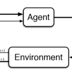
The process of Reinforcement Learning looks like this:

In Reinforcement Learning the computer (agent) takes actions within a given set of rules and possibilities (environment). Actions can lead to a positive encouragement (rewards) or negative encouragement (punishments). By taking an action, the agent is moving from one situation (state) to the next. Moreover, the environment holds, in case of chess, the rules of the game like physical size of the board and possible steps per type of piece. In Reinforcement Learning it’s about taking the best possible action or path to gain maximum rewards and minimum punishment in the future through observations in a specific situation.
In the chess game the state of the game would be the situation on the chess board, meaning where each piece is located on the board. This state gives us a possible action space for each piece, meaning all the possible actions at that moment for each piece on the board, of course keeping in mind the rules of the chess game. When the agent (player) moves a piece, the games reaches a new state. Which also means the possible actions for each piece on the board might change as well. Just like when we play chess ourselves, before the computer decides which move to make, it tries to predict what would be the most valuable move, i.e. which move would lead to winning the game as fast as possible.
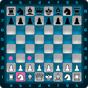
Let’s see how this would work for chess. The first image shows the start of the game, the first state, for the knight we show its actionspace, but of course each piece of the board has its own. Let’s assume the agent decides to move the knight. Leading to the second image, and second state, of the game. Also meaning the knight, and other pieces, have an updated actionspace.
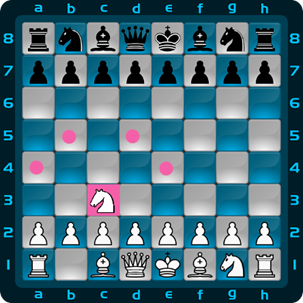
Of course, at the beginning of a game it can be quite difficult to predict which move would be the most valuable, but as the game progresses, this is becoming more and more clear and easier to predict. Something every chess player will recognize.
In Reinforcement Learning, the agent starts learning by using trial and error. It remembers which moves were made, how long the game lasted and what the outcome was. Like for ourselves, the more we play, the better we know what a good next move would be, giving the current state of the game. But unlike us, a computer can play games at ligthning speed and has a huge memory to remember every little detail.
In more technical terms, in Reinforcement Learning we can use a algorithm which uses the current state and action (next move) as input and expected reward as output. The goal is to find a suitable action model within the environment in which the agent increases the expected cumulative reward of the agent in the future. The expected cumulative future reward is expressed in a value function. Reinforcement Learning models update their value function by interacting with the environment, choosing an action, looking at the new state, looking at the reward, then updating. With multiple iterations the model will keep learning and we expect this value function to increase, meaning the agent will keep improving at playing (winning) the game.
Choosing the right Reinforcement Learning algorithm
In order to teach our agent to take the best actions in all possible states for acquiring the maximum reward over time, we need to choose a Reinforcement Learning Algorithm (RLA) with which our agent can learn what actions work best in the different states.
We call the collection of these preferred actions in the different states the policy of the agent. In the end, the agent should have a policy that will give her the highest lifetime reward. A large variety of algorithms to find the optimal policy exist and we will group them into three categories to make things understandable:
- Model Based
- Policy Based
- Value Based
Model Based
The first category is that of Model-Based RLA’s, where the algorithm uses a model to predict how the environment reacts to actions, thereby giving the agent ‘understanding’ of what her future state will be if she chooses for a particular action. In Model-Free algorithms, the agent will not have an explicit prediction of what her environment will look like after taking an action. So, although every RLA could be seen as a Machine Learning model for the agent to base its actions upon, the distinction between Model-Based and Model-Free is about whether an explicit (predictive) model about the future state is used or not.
Policy Based
Although not explicitly having an expectation of the future environment, some of these Model-Free algorithms can find the ultimate policy, based on searching for an optimal combination of states and wise actions to take in these states. These are called Policy-Based RLA’s. One of the most common algorithms of this sort is the Policy Gradient Method.
Value Based
Some algorithms go one step deeper than these Policy-Based algorithms by optimizing the expected future reward per state. In doing so, these Value-Based algorithms find the best actions to take in these different states, thereby having a collection of state-action combinations which ultimately make up the policy of the agent in her environment. So, Policy-Based and Value-Based algorithms seem very similar, but the main difference is that policies are stored and updated in Policy-Based algorithms, but in Value-Based algorithms the value function is stored and updated, from which the combinations of states and actions can be derived, and the policy thereby constructed. We will be using such an algorithm: Double Deep Q-Network (Double DQN).
Defining the SNAKE game
Now that we know what Reinforcement Learning is and how it teaches an agent to achieve goals by interacting with its environment, it is time to try it ourselves! Remember the game we used to play in the early 2000’s on our good old Nokia mobile phone? We have all been playing the nostalgic game Snake at least once in our life, right? The goal is simple: being a snake you navigate through a square playground looking for food. As you eat more food, the difficulty increases because your snake will grow longer, and you cannot crash into yourself. Snake is a good choice for a first introduction to Reinforcement Learning, because it lets us define the environment, agent, states, actions and rewards relatively simple.
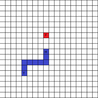
Our game environment can be defined as a grid of points, with a piece of food at a random coordinate in that grid. In our version of Snake there are no walls, which means that the only way the snake can die is by a collision into its own body. Our agent – the snake – is encoded by a list of coordinates that are covered by the snake, and the state is the current representation of the environment. The picture below shows an example of what the environment could look like. Where the F is food, H is the head of the snake and T is its tail.
For this article, we have experimented with different representations of the state, incorporating various sources of information such as the direction of the snake and the distance to the food. Additionally, we have experimented with adding spatial features extracted by convolutional filters. Convolutional filters extract spatial information of an image by multiplying regions of pixels in an input with weights that are learned by a neural network. This results in a feature mapping that encodes spatial information of the playground, like we will explain more in detail later on.
As the snake navigates through the environment, it can either move up, down, left or right. However, according to the rules of the game, the snake cannot move in the opposite direction of the current direction. Therefore, given the state, we can only take three out of four actions. This subset of actions is what we call the action space. Our goal is, given a certain state, to choose the action that maximizes the future lifetime reward, which can consist of multiple features. In the first place, our snake is rewarded when it eats food, and the score increases. Conversely, the snake is negatively rewarded when it collides into its own body. Additionally, we have included a small penalty to the reward when the snake moves further away from the food, and we added a small positive reward when the snake moves closer to the food. This encourages the snake to pursue eating food instead of only avoiding a collision.
It is very informative to play around with these rewards and punishments, since the result of your decisions on what to reward and what to punish might surprise you from time to time (actually, a lot of the times). For example, before introducing the small rewards and punishments for getting closer to or moving away from the food, the snake would sometimes run in circles in order to survive, thereby not scoring any points. On the contrary, a penalty for walking around for too long without eating, resulted in the snake wanting to commit suicide immediately to avoid “suffering” from walking around without eating. Taking into account how simple the game of snake is, imagine how hard it is to define good rewards and punishments in real life, to avoid “toxic” behaviour.
Now that we know what the actions, rewards and states in our situation are, it’s time to have a look at how we are going to incorporate this in a model that can be trained.
Optimizing Reinforcement Learning
By using a neural network with Python library Tensorflow we estimate the total future rewards of our possible actions given our state. So, given a set of input features, which is the current state, we are going to predict the future rewards given our possible actions. In other words, we are training our neural network by updating our Q function based on the reward for a given action. Such a neural network is called a Deep Q-Network (DQN). This Q-function is the prediction of total future reward for the agent, when choosing action a in state s. The formula representing the way the function is updated is called the “Bellman-equation” and given by:
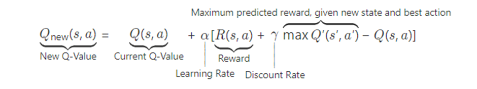
So, besides the Q function, the equation has parameter alpha as the learning rate of the algorithm that influences how fast the Q function is updated and therefore the rate at which the perception of the agent changes while learning her best actions. Reward function R shows the immediate reward of taking action a in state s. Discount rate gamma discounts future rewards that come after the immediate reward. This is necessary to reflect real life, in which a reward in the far future is most of the times deemed (slightly) less important than immediate reward. These hyperparameters alpha and gamma are set by the programmer before the algorithm is deployed.
By learning which actions give us the most future reward in which states, the agent can learn to effectively play snake.
We are going to train two different models with different input features/states in order to compare the performance and complexity of both versions.
Model V1 – a simple model
The first step we must take in building a DQN model is to define the features/states that we will use to predict the Q-values. This is one of the most important steps in setting up a Reinforcement Learning model as it yields all the information the model will use, such that giving too little information will result in a poor model performance. Nonetheless, we do not want to overcomplicate our first model and therefore choose fairly simple input features that contain signals about the location of the food and if there is a snake cell (i.e. her own body) beside the head of the snake.
For the first model we tried to keep the features as easy as possible to understand for our neural network (and ourselves 😉). The features used by this first model are as follows:
- X-coordinate of the food minus the x-coordinate of the snake’s head.
- Y-coordinate of the food minus the y-coordinate of the snake’s head.
- Dummy variable: if there is snake cell below head
- Dummy variable: if there is snake cell above head
- Dummy variable: if there is snake cell left of head
- Dummy variable: if there is snake cell right of head
Based on these features we give the snake information about the location of the food, and immediate danger of a certain choice based on the snake’s body. However, the snake does not have full information about her body and therefore cannot strategically choose actions to avoid being locked by her body later in the game.
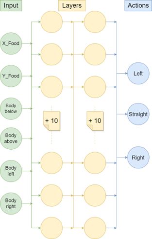
For this first version of the model, we insert fairly simple input features that consist of ‘which direction the food is’ and ‘if the snake’s body is near its head’, we do not want to overcomplicate our model. Therefore, we choose to build a neural network consisting of two layers with 16 neurons and end with a dense layer that forecasts the reward for each action. This neural network will then be used as our Q function.
Once the model is set, we want to train the model until it converges to an optimum, which means that we do not see the average reward improve anymore (enough) after a certain number of training iterations. We help the model converge quicker by giving example actions for 20% of the time. This way, the model has enough data about how to gain rewards such that these actions will gain higher Q-values.
For our first version of the model, we find that after around 500.000 training iterations, we don’t see the rewards improve anymore. This takes around 30 to 60 minutes of training, depending on the processor speed.
Model V2 – a more strategic model
As we chose our first model to be fairly simple, it could not look further ahead on the snake’s body to understand the full current state of the game and therefore the snake could be trapped easily inside its body such that it dies. To improve the model, we want to use a convolutional neural network to understand the full picture of the game such that it can make strategic choices so that it will not trap itself.
However, by using convolutional filters to understand the game’s image there is a tradeoff between simplifying the input by aggregating the pixels of the game, such that it will lose precision on the whereabouts of the snake’s body, and size of the network such that the network can understand the many pixels given by the image, where a too large size will make the model so complex that it will take very long to train.
To deal with this problem we create a combined network of the input features from the last model, that gives very precise information about dangers and directions, and combine them with the snake’s snapshot image such that it will give the snake more strategic insights about the state of the game.
In order to let the neural network understand the image, we transform the game into an array of shape: (game width, game height, 3). This array will then have an array with the length of three for each point in the snake’s map, that will be used to indicate if there is a snake body, snake head or food by using dummy variables. For example, if the pixel is filled with a snake’s body, the array will then be given by [1,0,0] and if there is food placed on the pixel the array will be given by [0, 0, 1]. Then, an example of what the full input array for the convolutional layers could be is given by:
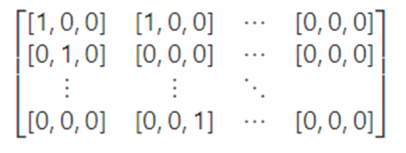
Now the input of the DQN model for this version will be a tuple with the state features of our first model’s version and the game state array for the convolutional part of the model. Because of this combination of two parts, it is a Double DQN.
As previously mentioned, the input of the model will be a combined input of model V1 on features and the image as converted to an array. Our model will first split our tuple containing both features by the features array and the convolution array. Once we have our separated array containing the snake’s game snapshot, we will let this go through two separate convolutional layers containing 8 filters, a kernel with size=(4, 4) and strides=2, where the padding is ‘same’ which makes sure that we also account for the border pixels in our model. After the input has gone through both convolutional layers, we will have extracted signals about the game like “there are a lot of body parts in the bottom right corner”, which can help the snake to stay away from there. Flattening this array of signals makes us able to use these signals in a normal dense layer. Next, after flattening the array, we use two dense layers of 256 and 64 neurons to further extract signals about the state of the game.
For the normal features we use one dense layer of 16 neurons to extract signals about immediate threats and the position of the food. The moment comes when we concatenate both the normal signals and our convolutional signals together such that we can use them simultaneously in a dense layer which will finally be used to predict the Q-values for each action.
Next, we train our multi-input model until the model converges to an optimum where the average reward is not improving anymore. As we have a much larger network containing convolutional filters, it will take the algorithm a lot longer to train. Again, we help the model by giving example actions for 20% of the time. Once the model has had a good amount of training loops (around 1 million iterations) this part can be removed to get more exploration observations and have more data to find a good strategy in the training data.
For this second version of the model, we find that it converges after approximately 5 million training iterations which take around 4-7 hours of training, depending on the processor speed.
Results
Finally, we come to the most important part of the project where we assess the performance of our models. To validate the performance, we want our models to play 100 games till the snake dies. Then we are going to compare the average score and the maximum score out of these 100 games to compare the models. Exploration is avoided, which means that the algorithm is never randomly choosing actions. These are the results:
| Score | V1 Model | V2 Model |
|---|---|---|
| Avg Score | 22.28 | 27.16 |
| Max Score | 47 | 72 |
For the model V1 the average score out of 100 games is 22.28 with a maximum of 47 which is not bad for the fact that this model is not able to lookout for threats ahead. However, incorporating the snapshot of the whole game into the model V2 gave us a significant improvement with an average of 27.16 and a maximum of 72. This shows us that the V2 model, the more strategic one, is indeed capable of determining strategies that look ahead to prevent the snake from getting trapped. However, the training time of this model was also significantly longer with 4-7 hours in respect to 30 to 60 minutes. Therefore, we really see a clear trade-off between performance and required training time to reach the optimum. In practice, this is always a hard decision as there is always a better solution, however the question arises: “Is it worth the time?”. From our first model’s output we saw that the performance was not bad either, so was it worth all the trouble to enhance it? For this article it definitely was!
Can you use Reinforcement Learning in your daily life?
Apart from interesting applications of Reinforcement Learning in games, these algorithms can also be used in business to improve how data can create value. Essentially, if decisions must be made about which actions to take given the current situation an organization is in, a Reinforcement Learning agent can be trained to make decisions or at least give advice on what the next best action should be.
One of these scenarios could be when a marketing team should decide whether to include a customer or prospect in a certain campaign and which offer or communication she should receive. For example, the agent here is the digital assistant of the marketeer, state the characteristics of the (potential) customer plus the timestamp and the actions are choosing between the different offers (or no offer at all) and communications. The environment, which is the real world, will give feedback such as clicks on weblinks, conversion or churn. The designer of the Reinforcement Learning Algorithm should then define the rewards corresponding to these events to steer the agent in the right direction for finding its optimal policy.
Another example could be that of personalizing the homepage on a website based on how a visitor is navigating through the website. The agent is not the visitor, but the digital content manager behind the website, who is choosing which banners to show on which places of the homepage (actions), given online navigation history (states) of the visitor and other information if the visitor is logged in with a profile or from cookies. If the visitor clicks on the shown banner, a positive reward is given by the environment, as this click shows the banner is relevant to the visitor and the homepage is being optimized for this type of visitor. The algorithm will find which actions (show a banner) link best to the possible states (collection of navigation history) to compose the policy.
Curious to see our code for both the Reinforcement Learning models, check out our other article!