Forecasting Dutch marriages after Covid-19
Geplaatst op: februari 21, 2022

The Python notebook and dataset is available from our Gitlab page.


What we Learned from Kaggle’s CommonLit Readability Prize
Geplaatst op: september 6, 2021

At Cmotions, we love a challenge. Especially those that make us both think and have fun. Every now and then we start a so-called ‘Project-Friday’ where we combine data science with a fun project. In the past we build a coffee machine with visibility, an algorithm for handsign recognition, a book recommender and a PowerBI escaperoom. A few months ago, we decided to join a Kaggle competition: the CommonLit Readability, for numerous reasons. First of all, for many of us this is the first time attending a Kaggle competition; high on many bucket lists. Not to mention we like to do more with textual data to get a deeper knowledge of NLP techniques. And last but not least, we like to help kids to read stuff that meet their profile.
In the CommonLit competition this question needs to be answered:
“To what extent can machine learning identify the appropriate reading level of a passage of text, and help inspire learning?”
This question arose as CommonLit, Inc. and Georgia State University wanted to offer texts of the right level of challenge to 3rd to 12th grade students, in order to stimulate the natural development of their reading skills. Until now, the readability of (English) texts, has been based mainly on expert assessments, or on well-known formulas, such as the Flesch-Kincaid Grade Level, which often lack construct and theoretical validity. Other, often commercial solutions also failed to meet the proof and transparency requirements.
To win a Kaggle competition…
Before we entered the competition, we did see some drawbacks. Often, a high rank in a Kaggle competition these days means combining many, many, many models to gain a bit of precision and a lot of rank positions – there’s not a lot of difference in accuracy in the highest ranked contenders. With the increase of predictive performance there’s a steep decrease in interpretability when combining the results of many models into a final prediction. Also, since this challenge is about textual data and we do not have many train cases, state of the art pretrained transformer models can be useful. Downside,these are complex and difficult to understand. Let alone when we combine multiple transformer models for our best attempt to win the competition…
What we did differently
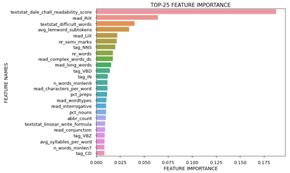
No mistake about it, when we join a competition, we’re in it to win it. But we wanted to maximize learning and explainability of our approach. Therefore, where we expected many others to focus on finetuning and combining transformer models, we’ve spent much of our available time on thinking of relevant features we could create that help in understanding why our model predicts one text is more complex to read for kids than another text. We brainstormed, read the literature and checked with our friends and family with positions in education. This resulted in an impressive set of 110 features -derived from the text. These features both include readability scales from the literature – Flesh reading ease, Flesh Kinraid grade, Dale Chall Readability score – as well as other characteristics we thought might help in explaining the readability of text – sentence length, syllables per word, abbreviations, sentiment, subjectivity, scrabble points per word, etcetera
Since we think understanding the why is as important as most predictive power, we followed this approach:
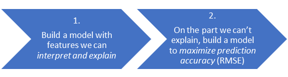
Model to explain readability
We started listing potential features and started creating them in the limited time we had available for this. After this feature engineering, we estimated XGBoost models to identify the most important features and included those features in a regression model. This approach resulted in valuable insights:
- About 55% of the variance in the readability score is explained [R2] by our features
- The well-known Dale Chall readability score is by far the most predictive scale
- Many extra features we derived help in predicting and explaining readability
Based on these results, we can think of ways how to help publishers, teachers and students how to write texts that are easier to read.
Model to boost predictions
Yet, we were not done with a model that is doing a good job in explaining. In the second stage, we explored if transformer models (BERT, Roberta, Distilbert) could help boosting our predictions. And it did! We knew these models, pretrained on huge amounts of textual data, are state of the art and excellent in many NLP tasks. Also in our case, RSME decreased from around 0.70 to 0.47 and the explained variance [R2] increased to 79%! After hyperparameter optimization a tuned Roberta Large with some advanced sampling was our best model.
And the winner is…
[spoiler alert!] No, we didn’t win this Kaggle competition. We ended somewhere in the upper half. To be honest, quite soon we knew that our approach would not be the one that would lift our bank accounts (the winner Mathis Lucka won $20K, congrats to him!). For this type of competition, the winner spends all time and resources on building many models and combining those, squeezing every last bit of predictive power out of the train data. For example, see the approach of the runner up. It should be noted however, that the winner, Mathis Lucka did use a bunch of models and ensembled those, but also had an original approach to involve smart new data (see his Kaggle post for details).
Even though we didn’t win, we enjoyed the competition very much and we’ve learned a lot. Also, we believe that our approach – have a model to interpret to explain the why and if needed add a booster to maximize predictions is a winning approach in many real life (business) contexts. (And we believe that an approach that ensembles 10+ transformer models is not ?). Therefore, we have already started translating what we learned in this Kaggle competition into something we can help others with to get and use more readable texts. Curious what exactly? Stay tuned and you’ll find out!


Can machine learning assess the readability of texts?
Geplaatst op: augustus 23, 2021
In May, we kicked off another Project Friday. This time, a group of seven Cmotions colleagues, of different origins and levels, came together. As always, the aim was to make a brilliant deliverable, to learn a lot, and (most of all) to have a lot of fun.
The first challenge was to come up with a topic, which would lead to a cool product that everyone is excited about. After brainstorming for a while, it was soon decided to enter the CommonLit Readability Prize (a Kaggle competition) focusing on the following question:
“To what extent can machine learning identify the appropriate reading level of a passage of text, and help inspire learning?”
This question arose as CommonLit, Inc. and Georgia State University wanted to offer texts of the right level of challenge to 3rd to 12th grade students, in order to stimulate the natural development of their reading skills. Until now, the readability of (English) texts, has been based mainly on expert assessments, or on well-known formulas, such as the Flesch-Kincaid Grade Level, which often lack construct and theoretical validity. Other, often commercial, solutions failed to meet the proof and transparency requirements.
From May to August ’21, we worked on developing a Python notebook that is able to assess readability scores better than current standards. We worked with a training dataset of about 3.000 text excerpts that were rated by 27 professionals. In these months, we investigated which features affect readability the most, which models and architecture are best to use, and how to tweak them. The name of our team? Textfacts!
Certainly, you want to know if we succeeded in predicting text readability better than existing solutions, right? Stay tuned and follow our blogs for our stories! Do you have any questions or do you want to know more about this cool project right now? Please click here to visit the competition webpage or contact us, via info@theanalyticslab.nl.

Creating an overview of all my e-books, including their Google Books summary
Geplaatst op: juli 9, 2021

If, like me, you are a book lover who devours books, you are probably also familiar with the problem of bringing enough books while traveling. This is where the e-book entered my life, and it is definitely here to stay. But how to keep track of all my e-books? And how do I remember what they’re about by just seeing their title? And, the worst of all problems, how to pick the next book to read from the huge virtual pile of books?
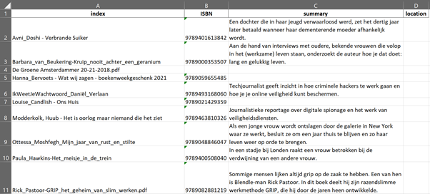
After struggling with this for years, I finally decided it was time to spend some time to solve this problem. Why not create a Python script to list all my books, retrieve their ISBN and finally find their summary on Google Books, ending up with an Excel file containing all this information? And yes, this is as simple as it sounds! I’ve used the brilliantly simple isbntools package and combined this with the urllib package to get the summary from Google Books. Easy does it! And the result looks like this:
If you’re curious on which book to read next now you’ve got such a nice list of all the books you’ve already read, you should definitely checkout our fantastic book recommender to help you find your next best book.
Take a tour in the code
Initialize
Let’s start by importing packages and initializing our input information, like the link to Google Books, the file path where my books can be found, and the desired name of the Excel file we want to create.
import os, re, time
import pandas as pd
from isbntools.app import *
import urllib.request
import json

# the link where to retrieve the book summary
base_api_link = "https://www.googleapis.com/books/v1/volumes?q=isbn:"

# the directory where the books can be found and the current list of books (if exists)
bookdir = "C:/MyDocuments/Boeken" #os.getcwd()
current_books = os.path.join(bookdir, 'boekenlijst.xlsx')
Check for an existing file with books
Next we want to check if we’ve ran this script before and if there is already a list of books. If this is the case we will leave the current list untouched and will only add the new books to the file.
# check to see if there is a list with books available already
# if this file does not exist already, this script will create it automatically
if os.path.exists(current_books):
    my_current_books = pd.read_excel(current_books, dtype='object')
else:
    my_current_books = pd.DataFrame(columns=["index", "ISBN", "summary", "location"])
Retrieve all books
Now we walk through all folders in the given directory and only look for pdf and epub files. In my case these were the only files that I would consider to be books.
# create an empty dictionary
my_books = {}

print("-------------------------------------------------")
print("Starting to list all books (epub and pdf) in the given directory")

# create a list of all books (epub or pdf files) in the directory and all its subdirectories
# r=root, d=directories, f=files
for r, d, f in os.walk(bookdir):
    for file in f:
        if (file.endswith(".epub")) or (file.endswith(".pdf")):
            # Remove the text _Jeanine_ 1234567891234 from the filenames
            booktitle = re.sub('.epub', '', re.sub('_Jeanine _\d{13}', '', file))
            booklocation = re.sub(bookdir, '', r)
            my_books[booktitle] = booklocation

print("-------------------------------------------------")
print(f"Found {len(my_books.keys())} books in the given directory")
print(f"Found {len(my_current_books)} in the existing list of books")
Only process the newly found books
We don’t want to keep searching online for ISBN and summaries of the books we’ve already found before. Therefore we will remove all books from the existing file with the list of books (if this existed). If there wasn’t already such a list, nothing will happen during this step.
# only keep the books that were not already in the list
if len(my_current_books) > 0:
    for d in my_current_books["index"]:
        try:
            del my_books[d]
        except KeyError:
            pass # if a key is not found, this is no problem

print("-------------------------------------------------")
print(f"There are {len(my_books.keys())} books that were not already in the list of books")
print("-------------------------------------------------\n")
Find the books online
For all the new books, we want to search for their ISBN using the book title (name of the file). Using this ISBN, we will try to find the summary of the book in Google Books.
# try to get more information on each book
i = 0
for book, location in my_books.items():
    print(f"Processing: {book}, this is number {i+1} in the list")
    isbn = 0
    summary = ""
    try:
        # retrieve ISBN
        isbn = isbn_from_words(book)
        # retrieve book information from Google Books
        if len(isbn) > 0:
            with urllib.request.urlopen(base_api_link + isbn) as f:
                text = f.read()
            decoded_text = text.decode("utf-8")
            obj = json.loads(decoded_text)
            volume_info = obj["items"][0]
            summary = re.sub(r"\s+", " ", volume_info["searchInfo"]["textSnippet"])
    except Exception as e:
        print(f"got an error when looking for {book}, the error is: {e}")
    my_books[book] = {"location":location, "ISBN":isbn, "summary":summary}
    i += 1
    # sleep to prevent 429 time-out error in the API request to get the ISBN
    time.sleep(5)
Store the list of books in Excel
Finally, we combine the existing list of books with all new books we’ve found and store this complete overview in the Excel file. We’re all done now and good to go.
# write to Excel
all_books = pd.DataFrame(data=my_books)
all_books = (all_books.T)
all_books = all_books.reset_index()
all_books = pd.concat([my_current_books, all_books])
all_books.to_excel(current_books, index=False)
It’s definitely not perfect yet, since the ISBN is matched using the title, which won’t be correct all the time, but I had a lot of fun creating this script, and I hope you’ll have fun using it!
Go to Gitlab to find the whole script and requirements.

Our package is live! Meet tortoise, your starting point for building Machine Learning models in Python
Geplaatst op: april 16, 2021

Machine learning in Python made easy in one simple package, check the source code here.
Starting to build machine learning models using Python can surely be overwhelming due to the endless possibilities that this open source tool offers. Therefore, we built a Python package that guides (junior) data analysts and scientists through all the steps involved in building machine learning models with easy to use functions.
What to expect from this package
The package consists of three classes (bundling of data and functions) which are based on the CRISP-DM (cross-industry standard process for data mining) model. These are
- Loading & Understanding Data
- Preprocessing Data
- Training Model
For each class, we have written functions that we think are crucial to properly execute that step of data modelling. For now, the package supports building classification models only. However, we are open source, so feel free to help us with adding other types of algorithms! Also a fourth class, containing functionality for model evaluation is still on our wish list, so feel free to help us there as well.
Now that the application of algorithms becomes more common within organizations, the role of Data Scientists transforms as well. More focus is often dedicated to the added value of the model and not necessarily to understanding the nitty gritty details on why the model is so good at predicting. Considering the huge amounts of data that an algorithm is able to process, it might not even be possible for humans to understand the details anymore. The trick is focusing on accuracy, while not losing explainability or the ability to put it into production.
So whereas Data Scientists used to be experts in statistics, currently the added value of a model becomes more important. And that is exactly why we want to help analysts with this package: to be able to add value to customers and their organization, with as little effort as necessary.
Getting Started
In order to get started we recommend starting at our GitLab Repository. For more information on installing the package, start with the README. For more information on working with the package we created a Tutorial that should get you acquainted with the package functions within 10 minutes.
Why we made this package
Last year, our former colleague Jeroen wrote an article in which different statistical analysis tools are compared. He concluded that open source tooling, as opposed to commercial tooling, is the way to go. The strength of these tools is that the communities behind them enable continuous development, making them more powerful, innovative and useful than existing commercial tools. Also, many commercial parties now integrate the ability to use open-source languages in their tools. By now, we observe that especially the use of Python is becoming more and more common practice within organizations. Looking into the near future, we dare to state that every data scientist needs to know at least R or Python.
The growing community also entails a growing number of packages, which can be cumbersome for a starting Data Scientist; where to start? Your primary goal as a Data Scientist is to add value to your customers & organization, so a tutorial on how to perform a particular algorithm on the Titanic dataset won’t do. We therefore decided to create a package which can be used as a starting point for building a model. Its focus is not only on the algorithms but on the whole process, which starts by determining where to add value!
Moreover, data science or analytics departments are becoming more important within organizations. Given that Data Analysts or Scientists from different teams might work on similar challenges using the same data, this raises a need for consistency and efficiency across different models. Therefore, it is convenient to have all the logic behind a model integrated within one package. By doing so, all data analysts can rely on the same ruling which means that models are becoming less dependent on the person who initially built it. So, if you get confused by the endless number of available packages or don’t feel like building a Python package for your organization yourself, we would strongly recommend using ours!
And obviously, as big fans of Python, it would be hypocritical to advocate the strength of the communities behind it if we would only free ride on the efforts of others.

Can you escape our “Power BI EscapeRoom”?
Geplaatst op: april 2, 2021

In these boring lockdown-times we are all desperately looking for ways to still interact with our colleagues, friends, and family in a fun and engaging way instead of yet another digital meeting. Not an easy task given the current circumstances, but we are an inventive bunch of people who love a good challenge.
So, we thought, where do fun, interaction and challenge meet each other? That’s right: in an Escape Room! And even better: in an Escape Room which can be played anytime, anywhere, with anyone you want. For free!
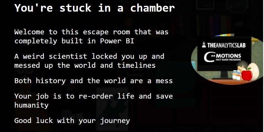
Power BI EscapeRoom
Of course, we could have chosen to simply search for an Escape Room online, reserve a spot and play that room. But since we are true and sincere data-loving nerds who love an extra challenge. We thought “why not try to build our own Escape Room using only the standard Microsoft Power BI functionalities”, and so we did! And boy, did we find what we were looking for! At Cmotions, when we create dashboards for our customers, we always try to make the best use of the navigation and interaction options in the data visualization tool at hand, to guide users through the dashboard as easy as possible. But naturally for this Escape Room we have deliberately made it a bit harder to navigate… We had so much fun in trying to figure out the best way to achieve what we wanted to create, limiting ourselves with only standard Power BI visuals (ok, the real experts might recognize a sneaky chiclet slicer, forgive us). For the Power BI users among our readers, hopefully this Escape Room will also inspire you to see the huge number of possibilities when using Power BI.
The Team
This was quite a challenge we’ve given ourselves, but outside of your comfort zone is where you learn! In this case we did not only learn a lot, but mostly, we had a whole lot of fun! Also, lucky for us, we had access to some of the most engaged data-lovers possible:

No navigation challenge is scaring this man. A true master of navigation, you will never get lost when he is around.

Looking for a storyline? Just talk to this creative woman. You will not only get a story, but you will also get completely sucked into this story. Just try our EscapeRoom and you will see what we mean.

No science fact is unknown to this man. In our EscapeRoom you get a chance to experience being inside his brain. We hope you can find your way out because that is not an easy task. Do not say we did not warn you…
Tell her a story and she sees it all happening in her brain. Walk around in her imagination as she brings the storyline to live in everything you see going on in our EscapeRoom.

A true lover of triple D. No dinosaur, disease or even dartboard can scare this man. See for yourself and you will know what we mean. Hopefully, he does not scare you away…

Be afraid all you little bugs, be very afraid. Because no other bug has ever been able to tell the story of running into this true bugmaster.
Let’s play!
All that is left for us now is to invite you into our brains by entering our Power BI EscapeRoom and have a whole lot of fun! You do not need any knowledge of data and/or Power BI to be able to experience this EscapeRoom. It is really open to everybody who loves a good puzzle. Please let us know your feedback, we would love to hear from you.
We helped Piet A. Choras escape his lockdown
Geplaatst op: maart 31, 2021

At Cmotions we usually really enjoy our weekly Fridays where we all come together at our headquarters. Mostly working for all our clients, but then at our own office. Which also gives us some space for our own projects, but mostly for simply being able to see and talk to each other and really feel like colleagues. It is a tradition we’ve all come to appreciate very much, which makes us feel like Cmotioneers and also the tradition we have been missing the most in this past covid-year.
But as consultants, we all have learned to be flexible and work with what we have as well. So why would this be any different. Therefore, we looked around us to see what we had at hand to “replace” our Friday feeling, even only for a little bit. We started out with our PowerBI EscapeRoom, which was not only a whole lot of fun to create but even more so to play! We can really recommend doing this with your teammates. It’s freely accessible for everybody and you don’t need to know anything about data or PowerBI to be able to play this EscapeRoom!
All the fun we had playing this PowerBI EscapeRoom made us crave for more fun, so we decided we wanted more! And why not use one of our very own hackathons as well: Escaperoom, the lockdown. This hackathon, which we created in 2018, was, suddenly, even more relevant now in 2021! In this hackathon our teams get the assignment to help free the mathematician Piet A. Choras, who was wrongly convicted for overfitting and has been in in lockdown ever since (boy, do we know how he feels!).
With a combination of logical thinking, a creative mind, our best friend Google and our even better friend the computer, the teams worked on all different sorts of assignments, ranging from visualization to math to analytics. Since the hackathon has a bring your own device concept, everybody was free to use the tools they preferred (and yes, even Excel is amongst these tools). The teams worked on solving all these different puzzles for a couple of hours, which in the end lead to a photo-finish, where the best predictive model won.

Even though nothing beats seeing each other in real life, this hackathon offered us a very fun afternoon, with a lot of competition, fun, knowledge sharing, teambuilding and learning of new skills. We finished with some online drinks and bites where every team could share what they did all afternoon. Which added even more fun, because this ranged from some very smart Python code, to a fancily coloured Excel and even some PowerBI fishes. No tool is left untouched during this afternoon.
Congratulations to Erik, Thijs and Kjeld, who won the eternal fame of winning this hackathon!

Does your team need a little energizer as well, for teambuilding, (fun) learning and just to have a little break from their regular workdays? We are more than happy to facilitate our hackathon at your company. We know, from our own experience, how much fun this will be! Please contact us at info@theanalyticslab.nl for more information.
Beginners guide to teamwork in Git
Geplaatst op: maart 26, 2021

My first encounter with Git was a disaster. I worked on a marketing intelligence project to standardize our model code. We asked a team of data scientists whether they had any useful code to share with us. Instead, they ‘helped’ us by introducing Git without too much explanation. A few days of struggling later, we were drowning in a sea of branches and merge conflicts and had barely written any code.
Luckily, this was not my last experience with Git. The next project my team came prepared with a neat collaboration structure and we are reaping the rewards ever since. This is what you need to consider if your team of coders is considering to collaborate on a project using Git.
What is Git
Git is basically an online folder structure with files filled with your code (e.g., Python files, notebooks, etc.), easily shared and updated. Git offers a great way to ensure everyone has the same version of code without the hassle of sharing and implementing snippets of code with your colleagues. The main purpose of Git is version control, which means you can easily access previous versions of the project. Git is also very useful for code deployment.
Choose your Git
There are a few variations out there, most popular are Gitlab and Github . Both offer private repositories for free. We chose Gitlab for our project. You can find some extensive documentation here and here. Whichever platform you choose, you need to install GIT on your computer.
How to use Git
Git is mainly used from the command line, where you use specific commands to synchronize the changes you make on your computer with the changes others make. You can send (“push”) the changes you made locally to the shared online environment, you can download (“pull”) the changes others have made to your computer, and Git makes sure these changes are automatically integrated without interference.
Choose a collaboration structure
If you use Git to work together on a project, i it is useful to think about how to add your individual contributions to the project without overwriting other code or breaking down the project as a whole. Especially with programming projects, there is a chance you can ruin a working project by introducing bugs when you push your code, a good collaboration structure can prevent that.
A common approach is to use different branches (i.e. versions of your project) for different purposes. A branch is a copy of project code, meant to be used as a specific version. For example, a master branch with the latest production-proof version of the project and a development branch that can be used to add and test new features to the code. On our last project we used the following structure (based mainly on this and this article) as depicted in the figure below.
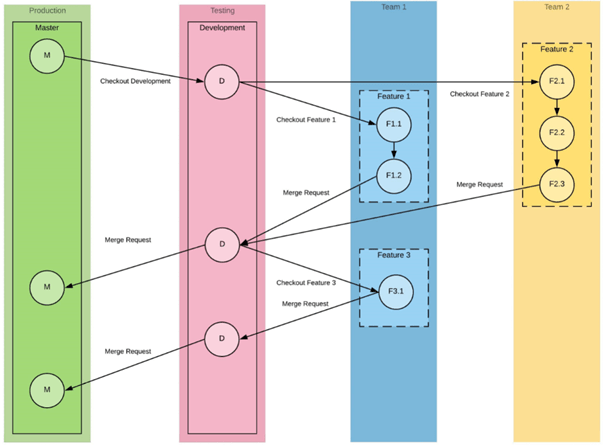
The way of working was as following:
- Create a feature branch by making a copy of the development branch. Name it after the feature you are going to build.
- Pull the feature branch to your computer.
- Add new code to the project.
- Push your feature branch to the online project.
- Create a merge request to merge your feature branch with the development branch.
- Peer review the merge request and merge it with the development branch. The development branch now contains your new code.
- Repeat step 1-6.
As soon as the development branch with the new feature is tested and stable, merge the development branch into the master branch. In next segment we’ll provide you with the necessary command line code to follow this structure.
Getting started
Now put your collaboration structure to practice.
- Make sure Git is installed
- Go to gitlab.com and add a project
- Add a development branch to your project
Clone the project
Every team member can clone this repository and contribute to it by opening a command prompt and type the following commands:
# go to the directory where you want to create a local copy of the project
cd your_directory

# copy the whole folder with the project from git to your computer
git clone https://gitlab.com/name_of_your_project.git

# go to the folder of your project
cd name_of_your_project
You now have a local copy of the project. From now on, we can just follow the steps in our way of working. In this example, you’ve named your git project ‘new_project’ and the feature you are working on will be named ‘new_feature’.
Create a feature branch
Go to gitlab.com/new_project and create a new branch ‘new_feature’. Of course, you should give it a more meaningful name that corresponds with the purpose of the feature. For example ‘imputation_function’. The purpose of the branch can also be something else than a feature. For example, a bug fix. If you already have a branch you are working on, just skip to step 2.
Pull the feature branch
Open a command prompt and type:
# go to your project directory
cd your_directory/new_project

# sync your project locally
git pull

# switch to the new feature branch
git checkout -b new_feature origin/new_feature
You now have a local copy of your new feature, currently still the same as the up to date development branch.
Add new code or change existing code in the project
Add/modify files in your project locally. For instance, in our project new features were often a piece of code (a new function) added to a python file. But it can also simply be some modifications to a README for instance. Make sure you test your new code (if applicable) and everything works as expected and no other parts of the code broke down due to the changes you’ve made.
Push your feature branch
As soon as your feature is complete, you can then commit and push your code. From this moment on, all your team members can see all the changes you’ve made in the feature branch. Next, share your new feature with your colleagues by submitting a merge request with the development branch. Your team can review the feature on gitlab.com and either accept or decline the merge request. First, push the changes you made locally to your feature branch to the shared online environment.
In your command prompt:
# add all changed documents (if you want you also only specifically add a single (set of) document)
git add .

# commit all the changes you made, don't forget to add a meaningful and short commit description
# each commit will be visible as a single change, the smaller the commit, the easier the rollback will be when something produces errors
git commit –m “added imputation techniques to data_cleaning.py”

# push all existing commits to the online version of your new_feature branch
git push origin new_feature
Create a merge request to the development branch
Check the Gitlab repository to check whether your branch is uploaded. When successful, click on Merge Requests > New merge request, add the description and choose to merge your new branch with the development branch. Delete the new_feature branch after merging (checkbox) to keep your project clean and prevent “stale” (old/unused) branches..
Peer review the merge request
After submitting, tag a colleague to review the request and either decline and provide feedback or directly merge your request into the development branch, thereby making it available in project.
You now have successfully contributed to the project! Hopefully…
Tips & tricks to smoothen the collaboration
Use .gitignore
Not every file in your project has to be shared and merged in Git. For example, if you use jupyter notebooks to test your code or have some datasets present, just place a file ‘.gitignore’ in your project and write down all the files and/or extensions Git should not synchronize. For example: ‘*.ipynb’ to ignore all jupyter notebooks in your main folder or /Data to ignore all files in the folder named Data.
Use merge requests
Creating merge requests is a neat way to be aware of all admissions of new code and a moment to peer review. To avoid that your teammates merge their branches instantly with development – or even worse, the master branch – you can RESTRICT this possibility in their roles.
How to handle merge conflicts
When you and your colleagues made changes to the same lines of code, and both push your changes, a merge conflict will occur. Git does not know which changes are “the best”. Merge conflicts often cause headaches, so in short the best way to resolve them:
- Type “git status” in the command line, and look for the file that is conflicted
- Open the file in a text editor
- Look for the “<<<<<<<” in the file
- The two conflicting codeparts are separated by “ =======”, remove this and the option you do not want to keep
- Remove the lines with “<<<<<<< HEAD” and “ >>>>>>> ‘YOURBRANCHNAME’“
Then you can proceed normally with a merge request or a push (step 4 above).
Drop your own changes and pull new changes
Sometimes a colleague has made changes on the same piece of code that you were working on, and you want to “drop” the changes you made to prevent merge conflicts. The easiest way to do this is to use the command “git stash”. This command stores all changes you made and restores your code to the last pulled version. Now you can pull the changes without conflicts! And rest assured, if you want your changes back this is still possible. For more details about stashing look here.
I hope this article has made you enthusiastic on the use of Git for your projects. In any case after reading this article your introduction to Git is likely to be less disastrous as my first attempt.

After reading this still feel like you would like some guidance when it comes to start using Git? Just reach out to us on info@theanalyticslab.nl and we can tell you all about the Git training we give.

Curious on one of the projects we collaborated on using Git, check out our very own Python package on Gitlab (available through a pip install): tortoise.


Book recommender
Geplaatst op: maart 22, 2021
Almost every day we go online we encounter recommender systems; if you are listening to your favorite song on Spotify, binge watching a TV show on Netflix or buying a new laptop on Amazon. Although we all know these recommendation engines exist, it is less known what algorithms lie behind such recommendations. To get a better understanding of the algorithms used in recommender systems we decided to build a recommender ourselves! With COVID-19 making us more housebound than ever, a topic for our recommendation engine was quickly found; we decided to build a book recommender using Python. Although there are ready-to-use packages to build recommender systems (such as Surprise) we decided to built or own recommendation system. We did this because our goal was to understand how a recommendation engine works rather than just have a book recommender. Moreover, we wanted to be able to control the specifications of the variables used in our engine and wanted to avoid the black box. In this notebook we explain step-by-step how we built our recommendation engine.
Our notebook contains of the following steps:

Data
A lot of recommenders have been build using English data sources such as the data scrapped from goodreads.com. We decided that we will use a new source and create a Dutch recommender instead. The data that we are using was obtained from a Dutch book review website. The source data is not made available. We obtained two data files: book data and rating data. The book table includes the information about the book itself such as:
- the name of the book,
- the author of the book
- book_id
The ratings table consists of the scores that users gave to the book. It includes:
- the book_id
- user url (unique per person)
- the rating (ranging from 1, did not like the book to 5, loved the book).
We will need to combine the two tables in order to build our recommender.
# import packages
import pandas as pd
import numpy as np
import matplotlib.pyplot as plt #creating
import random
from sklearn.preprocessing import LabelEncoder
from sklearn.metrics.pairwise import cosine_similarity
from scipy import sparse
from ftfy import fix_text
import hashlib  #to hash personal data
from six import ensure_binary #to hash personal data
# import ratings and books data into dataframes
books = spark.sql("select * from bookies_txt").toPandas()
ratings = spark.sql("select * from reviewies_txt").toPandas()
#Hashing personal data
ratings.Reviewer_url = ratings.Reviewer_url.apply(ensure_binary).apply(lambda x: hashlib.md5(x).hexdigest())
books.head()
ratings.head()
However, prior to merging the books' data with the ratings we investigate whether or not books are rated more than once. If the book is rated only by 1 or 2 people it is incredibly unlikely that it will be present in the output of a recommender, and will only slow it down. As you can see from the graph below, most books have indeed only been rated a few times. Thus, we will remove all books that have been rated at most 3 times. Though, we want to make sure that after we do this, we still have enough data to work with.
df = ratings.groupby('Book_id').agg({'Reviewer_url':'count'}).reset_index()
plt.figure(figsize=(8,6))
plt.hist(df['Reviewer_url'], range=[0, 50], bins = 50, ec='black')
plt.xlabel('Book ratings')
plt.ylabel('Number of people')
display()

min_book_ratings = 3

more_than_3_reviews = ratings[{'Reviewer_url', 'Book_id'}].groupby('Reviewer_url').agg({'Book_id':'count'}).reset_index()
more_than_3_reviews_list = more_than_3_reviews['Reviewer_url'].loc[more_than_3_reviews['Book_id']>=min_book_ratings]
book_review_popular = ratings.loc[ratings['Reviewer_url'].isin(more_than_3_reviews_list)]
print('Number of unique books: ',book_review_popular['Book_id'].nunique())
Based on this exercise, we are left with 105,459 books, which is a decent number of items, so we will continue building the recommender. We can now proceed with merging of the book data to the ratings data.
One interesting observation that we had by simply browsing the hebban website, is that they do not combine book versions. Thus, if say the book was originally published in 2015 and then re-published in 2020, we will have two different web pages with two sets of ratings. This occur with roughly nineteen thousand books, thus we will aggregate these books to make sure that in the recommender only one version of the book will be visible. Another little issue that we spotted in the data was related to the encoding, this was fixed using the fix_text function.
books_ratings = pd.merge(left =book_review_popular, right =books ,  on = 'Book_id' , how = 'inner')

#Aggregating book versions
books_new_id = books.groupby(['Book_name','Author_name']).agg({'Book_id':'max'}).reset_index().rename(columns = {'Book_id':'New_book_id'})
books_ratings_new_id = pd.merge(left = books_ratings, right = books_new_id, on = ['Book_name','Author_name'], how = 'inner')
books_ratings_new_id = books_ratings_new_id.drop(columns = 'Book_id')

#fixing encoding
books_ratings_new_id['Reviewer_url'] = books_ratings_new_id['Reviewer_url'].str.strip('"').apply(fix_text)
books_ratings_new_id['Rating'] = books_ratings_new_id['Rating'].str.strip('"')
books_ratings_new_id['Book_name'] = books_ratings_new_id['Book_name'].str.strip('"').apply(fix_text)
books_ratings_new_id['Author_name'] = books_ratings_new_id['Author_name'].str.strip('"').apply(fix_text)

books_ratings_new_id['Reviewer_url'] = books_ratings_new_id['Reviewer_url']
books_ratings_new_id['Rating'] = books_ratings_new_id['Rating'].str.slice(start=2)
books_ratings_new_id['Book_name'] = books_ratings_new_id['Book_name'].str.slice(start=2)
books_ratings_new_id['Author_name'] = books_ratings_new_id['Author_name'].str.slice(start=2)

books_ratings_new_id['Rating'] = books_ratings_new_id['Rating'].astype(int)

books_ratings_new_id=books_ratings_new_id.drop(columns=['Book_url','Author_url', 'Publish_date'])
books_ratings_new_id.head()
After merging and aggregating we are left with a dataset that includes 94.836 books and 37.673 people who rated these books. This is a sufficient amount of data to proceed. We have removed the user names from the overview above, to protect the identity of the raters. We have now prepared the data and the resulting dataframe consists of rows for every single rating-book combination. Prior to building the recommender itself, we inspect the data for any anomalies that might influence the design of our recommendation engine.
print('Number of unique books: ',books_ratings_new_id['Book_name'].nunique())
print('Number of unique raters: ', books_ratings_new_id['Reviewer_url'].nunique())
print('Number of unique authors: ', books_ratings_new_id['Author_name'].drop_duplicates().shape[0])
Data Exploration
Looking at the distribution of book rating. Interestingly, most ratings are positive, with the majority being rated with 4. This implies that the recommender will be biased towards books that are rated positively. Hence, to get the best output from the recommender, the input should also consist of books that the user would rate highly themselves.
# distribution of rating scores
bins = np.arange(0, books_ratings_new_id['Rating'].max() + 1.5) - 0.5
plt.hist(books_ratings_new_id['Rating'], bins)
plt.xlabel('Book ratings')
plt.ylabel('Number of people')
plt.show()

One of our initial ideas was to create a recommender at an author-level as well as book-level. However, as we can see from the graph above, most people only rate a single book by the author. Thus, we do not have the evidence that aggregating the data as an author level will give interesting results.
#Distribution of times author is rated
df = books_ratings.groupby(['Author_name']).agg({'Rating': 'count'})
plt.hist(df['Rating'], range=[1, 20], bins = 20)
plt.xlabel('How many times the author is rated')
plt.ylabel('Number of people')
plt.show()

Recommendation engine
Now that our data is ready, we can finally get to building the recommender itself. We created a book recommender which is based on the collaborative filtering technique (https://predictivehacks.com/item-based-collaborative-filtering-in-python/). Hereforth, we refer to the data points which correspond to individuals who rated books as people and to the one using the recommender as the user. The algorithm returns the best-rated books by the people who have most similar taste to the user. The similarity is assessed by comparing the rating scores of the user to those of all people in the data. The recommender takes as input the ratings of the user and the percentage of the data to be used for prediction. The predictions should include three columns: the title of the book, the author of the book and the rating itself. It is advised to rate the books on the scale from 1 to 5, where 1 is 'I did not like the book' and 5 'I loved the book'. Further there are three optional inputs: number of books to return, number of users to compare and the number of reviews. The Number of books to return refers to the number of recommended books that a user wishes to be displayed. This variable is set to 10. The number of users to compare to is the number of users that will be selected based on the similarity measurement in order to create the 10 (or any other number that the user selects) recommended books. The final input, namely the number of reviews refers to the minimum number of reviews that the book should have in order to be displayed. This is referred to the number of reviews by the most similar people. If this input is kept at 1, the recommender is heavily influenced by outliers. However if the number of users to compare to is kept low while the number of reviews is kept high, it is possible that less than the desired number if books will be returned since there won't be enough books in common.
The training data is pre-processed which includes cleaning and reshaping. Thus the training set consists of a matrix which has unique people as rows, unique books as columns and book ratings as elements. In case that the person had more than one rating of the same book, only the latest is taken into account. If a person did not rate a book then the score is set to 0. Since the lowest rating for the book is 1, there is no confusion between the books that were not rated and those that were rated poorly.
The recommender consists of the following steps:
- Transforming and appending the information supplied by the user to the training data.
- Creating the references for both books and raters equal to their row/column, later to be used to be able to find back the books/raters in the data
- Create an empty sparse matrix equal in dimensions to the data and fill it with the book ratings. We chose to work with sparse matrices since most people have rated but a few books, so most elements of the matrix are in fact zeros. This is not necessarily needed, but it greatly improves the speed of calculation.
- Create sparse vector with the ratings of the user.
- Quontify the similarity between the user and all other people in the data. This is done wuth the cosine similarity.
- Now that we calculated the similarity, we can select top 100(of the number specified by the user) people in the training data who had most similar books ratings to the user, based on cosine similarity. At this step we also filter the points based on the minimum number of books that need to match.
- Select the books that were rated by the top 100 but not by the user him/herself and calculate the average rating of the books based on the data of the top 100.
- Select the number of the top-rated books that the user wishes to receive and display the results.
def recommender(ratings_of_user, sample_size, Number_of_books_to_return = 10, Number_of_users_to_compare = 100, NrReviews = 1):

  ###Step 1: Transforming and appending the information supplied by the user to the training data
  books_ratings_sample = books_ratings_new_id.sample(frac = sample_size).copy()
  data_to_restructure = books_ratings_sample[{'Book_name', 'Rating', 'Reviewer_url', 'New_book_id'}].append(ratings_of_user[{'Book_name', 'Rating', 'Reviewer_url', 'New_book_id'}]).copy() #appending user for whom the prediction is to be made
  df = data_to_restructure.groupby(['Book_name', 'New_book_id','Reviewer_url']).agg({'Rating':'count'}).reset_index()
  data_to_pivot = pd.merge(left = data_to_restructure, right = df , on =['Book_name', 'New_book_id','Reviewer_url'] , how = 'inner')
  data_to_pivot_unique_rows = data_to_pivot.loc[data_to_pivot['Rating_y']==1].copy()

  ###Step 2: Creating the references for both books and raters equal to their row/column, later to be used to be able to find back the books/raters in the data
  #enumerate books and reviewers
  lb_make = LabelEncoder()
  data_to_pivot_unique_rows.loc[:,'Book_code']=lb_make.fit_transform(data_to_pivot_unique_rows['New_book_id'])
  data_to_pivot_unique_rows.loc[:,'Reviewer_code']=lb_make.fit_transform(data_to_pivot_unique_rows['Reviewer_url'])

  #unique users
  unique_users = data_to_pivot_unique_rows['Reviewer_url'].sort_values().unique()
  #unique books
  unique_books = data_to_pivot_unique_rows['New_book_id'].sort_values().unique()

  ###Step 3: Create an empty sparse matrix equal in dimensions to the data and fill it with the book ratings
  #matrix with unique users as rows and unique books as columns
  empty_matrix = np.zeros((unique_users.shape[0],unique_books.shape[0]),dtype='uint8')

  #fill the empty matrix with corresponding ratings per user per book
  for i in data_to_pivot_unique_rows.itertuples():
    empty_matrix[i.Reviewer_code, i.Book_code] = i.Rating_x

  ###Step 4: Create sparse vector with the ratings of the user
  #the index of a the person to predict in an array
  user_to_predict = ratings_of_user.Reviewer_url.iloc[1]
  index_predict = np.where(unique_users == user_to_predict)[0][0]

  ###Step 5: Quontify the similarity between the user and all all other people in the data.
  A_sparse = sparse.csr_matrix(empty_matrix)
  similarities = cosine_similarity(A_sparse, sparse.csr_matrix(empty_matrix[index_predict]))

  ###Step 6: Select top Number_of_users_to_compare people in the training data who had most similar books ratings to the user
  similar_users = pd.DataFrame({'Users' : unique_users,
             'Similarity_index' : similarities.flatten()})

  #remove a person for whom the predictions were made; sort and grab top 10 most similar users
  similar_users = similar_users.drop([index_predict])
  similar_top10_users = similar_users.sort_values('Similarity_index', ascending = False).head(n=Number_of_users_to_compare+1)

  ###Step 7: Select the books that were rated by the top Number_of_users_to_compare but not by the user him/herself and calculate the average rating of the books based on the data of the top 100.
  Books_of_similar_users = data_to_pivot_unique_rows.loc[(data_to_pivot_unique_rows.Reviewer_url.isin(similar_top10_users.Users)) &
                                                         (~data_to_pivot_unique_rows.New_book_id.isin(ratings_of_user.New_book_id))]

  Book_rated = Books_of_similar_users.groupby('New_book_id').agg({'Rating_x':['mean', 'count']}).reset_index()
  Book_rated.columns = ['New_book_id', 'Rating_mean', 'Rating_count']
  books_temp = Book_rated.sort_values('Rating_mean', ascending = False).reset_index()
  Books_to_present = pd.merge(left = books_ratings_sample, right = books_temp, on = 'New_book_id', how = 'inner')
  Books_to_present_unique_records = Books_to_present[['Book_name', 'Author_name', 'Rating_mean', 'Rating_count']].drop_duplicates().copy()
  Books_to_present_unique_records.loc[:,'author_score'] = Books_to_present_unique_records.groupby(['Author_name'])['Rating_mean'].rank(method ='first', ascending=False)

  ###Step 8: Select the number of the top-rated books that the user wishes to receive and display the results.
  Books_to_return = Books_to_present_unique_records.loc[(Books_to_present_unique_records.author_score==1) & (Books_to_present_unique_records.Rating_count >=NrReviews)].sort_values('Rating_mean', ascending = False).head(n=Number_of_books_to_return).copy()
  Books_to_return2 = Books_to_return.drop(columns=['author_score', 'Rating_count'])
  return Books_to_return2#[['Book_name','Author_name']]
Now, let us demonstrate how the recommender works. We will use the data of one of our colleague (Anya) and use her ratings to derive two recommendations. We make a dataframe with her ratings and combine it with the books data in order to obtain book identifiers.
books = ['De reisgenoten','Diep Werk','Emma','De beer en de nachtegaal','Good Vibes, Good Life','Pilaren van de aarde / De kathedraal','De pest','The Master and Margarita','1q84 - de complete trilogie','To kill a Mockingbird', 'Gone with the wind']
authors = ['J.R.R. Tolkien','Cal Newport','Jane Austen','Katherine Arden','Vex King','Ken Follett','Albert Camus','Mikhail Bulgakov','Haruki Murakami','Harper Lee','Margaret Mitchell']
ratings = [4,5,5,4,4,3,4,5,5,5,5]
name = 'Anya'
Anya = {'Book_name':books, 'Author_name': authors,  'Reviewer_url':name, 'Rating':ratings}
Anya_df = pd.DataFrame(data=Anya)
Anya_df_ready = pd.merge(left = Anya_df, right =books_ratings_new_id[['Book_name','Author_name','New_book_id']] , on = ['Book_name','Author_name'] , how = 'left').drop_duplicates()
Below you can see that not all books which she supplied were found in the data. Sadly a book by Vex King 'Good vibes, good life' was not found. It is important to have a sufficient number of books to be able to produce a good recommendation. Perhaps we should have given a set of books to rate, which are definitely in the data. However such an approach would make it less engaging for the user. Not to mention, our recommender is biased towards positively rated data, thus the set our books that the person is rating should include the books that they enjoyed.
Anya_df_ready
As mentioned before, we run a test with the different parameters:
- x = the number of most similar people
- N = the minimum number of times a book must be reviewed by the top x people to be part of the recommendations
To be less sensitive for outliers in our recommendations we wanted to increase the number of times a book must be reviewed (N). We can only do this if we also increase the number of reviewers we take into account (x). We tested with values for N from 1 to 3 and therefore we must vary x between 10 and 100 to have enough recommendations.
Luckily, our colleagues wanted to act as a test group for this experiment. Based on their recommendation of 10 books they choose themselves, we created multiple recommendation lists per person with the book recommender. By marking their favourite list, we can give you our opinion on the best parameters.
First we have to remark that our colleagues did not all agree on the best parameters. In general we can say it's better to recommend books which are reviewed more than once by your top x group. A higher N is not always better as our colleagues marked the recommendations with N=3 as 'too general' and 'only bestseller'.
Choosing the preferred values for N and x depends on the tradeoff that one makes between receiving reliable recommendations that might be quite obvious or receiving less stable recommendations that are more surprising. Thus, someone that wants to receive a list with new and surprising books will have to settle for slightly less reliable recommendations. With our data and in our test group the options N=2 and X=50 plus N=2 and X=100 where the best options. Let's have a look at Anya's lists with those parameters.
print(recommender(Anya_df_ready, 1, Number_of_users_to_compare=50, NrReviews=2).to_string(index=False))
print(recommender(Anya_df_ready, 1, Number_of_users_to_compare=100, NrReviews=2).to_string(index=False))
The average rating is better, as for most colleagues, with a higher x (4.97 versus 4.50). We see the same behaviour in the output for Anya. Hereby we have to remark that is depends on your taste. When you tend to enjoy reading the bestsellers, you should get the best results with a small x.
Our team is very proud to have been able to gather our own data and build a book recommender from scratch. It was a journey which we started wanting to practice our Python skills in a completely different settings. In fact the most interesting part was deciding what variables to use. In fact, the first decision we had to take before we even started building the recommender. We described above how we had to omit the books that were rated by only a couple of people. Secondly, we put a lot of thought and effort into figuring out the best number of people to be compared with and the overlap between the books' ratings. As you saw, we don't actually have an answer to what is the best combination of these parameters and instead we think that playing around is best depending on what kind of books you would like to receive.
Would we change anything about the journey? Perhaps if we were to create our recommender from scratch, we would look for the data that is not positively skewed and would include book genres. This would allow to tailor predictions to the wishes of the user. Another data source can solve this.
